---
title: "Fairness in Algorithmic Decision-Making"
execute:
enabled: true
jupyter: python3
---
```{python}
import numpy as np
import pandas as pd
import matplotlib.pyplot as plt
import seaborn as sns
from scipy import stats
import warnings
warnings.filterwarnings('ignore')
sns.set_style('whitegrid')
plt.rcParams['figure.figsize'] = (7, 4.5)
plt.rcParams['font.size'] = 12

DATA_DIR = 'data'
np.random.seed(42)
```
> *Both teams did the arithmetic correctly. Both teams were right.*
In 2016, two teams of analysts looked at the same dataset and reached opposite conclusions about whether the algorithm scoring it was fair. They had chosen different mathematical definitions of fairness --- and the definitions were mutually incompatible.
This chapter is about that fact. There are several reasonable mathematical definitions of "fair," they disagree on real data, and which one to satisfy is a values choice no algorithm makes for you. Chapters 1--19 built a toolkit for turning data into decisions. Fairness is where the limits of the toolkit become impossible to look away from.
The chapter is enrichment material. There are no quiz problems and it is not on the final exam. The goal is to give you the vocabulary you need to read a fairness debate --- in a newsroom story, a courtroom filing, a tech-company report --- and tell what each side is and isn't claiming.
## Why fairness, and why now
Judges in Broward County, Florida set bail using a recidivism risk score called COMPAS. A 2016 investigation by *ProPublica*^[Angwin, J., Larson, J., Mattu, S., & Kirchner, L. (2016). "Machine Bias." *ProPublica*, 23 May 2016. <https://www.propublica.org/article/machine-bias-risk-assessments-in-criminal-sentencing>] argued the score was biased against Black defendants: among defendants who did *not* go on to reoffend within two years, Black defendants were roughly twice as likely as White defendants to have been labeled high risk. Northpointe, the company that built COMPAS, responded that the score was *equally accurate* across groups: among defendants labeled high risk, about the same fraction in each group actually reoffended.^[Dieterich, W., Mendoza, C., & Brennan, T. (2016). "COMPAS Risk Scales: Demonstrating Accuracy Equity and Predictive Parity." Northpointe Inc.] Both claims were correct on the same data. They were claims about different things.
The COMPAS dispute is one instance of a larger pattern. Algorithmic decisions about people now sit inside choices about who is offered a job interview (résumé screening), who gets a loan (credit scoring), who is flagged for a welfare-fraud investigation, what a student's grade should be when the exam is cancelled (the UK's 2020 A-level algorithm), and what dose of pain medication a hospital patient is offered. The cost of a mistake is no longer "the regression has an $R^2$ of 0.78." It is whether someone goes to jail awaiting trial, sees a mortgage offer, gets a callback.
Existing US civil-rights statutes --- the Civil Rights Act, the Equal Credit Opportunity Act, the Fair Housing Act, the Americans with Disabilities Act --- define *protected attributes* on which a hiring, lending, or housing decision is forbidden to discriminate. The 2020s added algorithm-specific obligations on top of them: the EU AI Act (2024), New York City's bias-audit law for employment tools (2023), and the EEOC's 2023 guidance reaffirming the four-fifths rule for algorithmic selection.
Protected attributes are *legally specified*. They are not the only attributes a person has. They are not always the ones driving the disparate outcome. But they are the ones the law tells you to check. Barocas and Selbst^[Barocas, S., & Selbst, A. D. (2016). "Big Data's Disparate Impact." *California Law Review*, 104(3), 671--732.] are the standard reference for how US antidiscrimination doctrine maps (often awkwardly) onto algorithmic decisions.
:::{.callout-note collapse="true"}
## Going deeper: the 2020s regulatory landscape
- *US protected-class statutes (existing):* Civil Rights Act (Title VII, employment), Equal Credit Opportunity Act (credit), Fair Housing Act (housing), Americans with Disabilities Act. The 1978 Uniform Guidelines on Employee Selection Procedures established the *four-fifths rule* --- a selection rate for any group at least 80% of the rate for the top-selecting group --- as a screening benchmark. The EEOC's 2023 guidance^[U.S. Equal Employment Opportunity Commission (2023). "Select Issues: Assessing Adverse Impact in Software, Algorithms, and Artificial Intelligence Used in Employment Selection Procedures Under Title VII of the Civil Rights Act of 1964." 18 May 2023.] reaffirmed the rule's application to algorithmic selection.
- *EU AI Act (Regulation 2024/1689, in force from August 2024).*^[Regulation (EU) 2024/1689 of the European Parliament and of the Council of 13 June 2024. <https://eur-lex.europa.eu/eli/reg/2024/1689/oj>] Prohibits some uses outright (social scoring by public authorities; real-time remote biometric identification in public spaces, with narrow exceptions). Subjects "high-risk" systems in employment, credit, insurance, education, and law enforcement to bias-monitoring, data-governance, and human-oversight obligations.
- *US state and local.* New York City Local Law 144 (in force January 2023) requires an independent bias audit before an automated employment-decision tool can be used. Colorado SB 24-205 (signed May 2024) became the first US state comprehensive AI statute. The federal executive-branch picture is in flux.
:::
When told an algorithm produces racial disparities, a first instinct is to remove race from the model. We will see in a moment why that does not accomplish what it sounds like it does --- but first, some notation.
## Setup and notation
Throughout the chapter, $x$ is the vector of features available about an individual, $y \in \{0, 1\}$ is the true outcome the decision concerns (did the defendant reoffend? did the borrower default?), $\hat y$ is the model's binary prediction, and $a$ is the protected attribute. We keep $a$ binary in the worked examples ($a = 1$ for the historically disadvantaged group, $a = 0$ for the historically advantaged group), with the understanding that the definitions generalize to more than two groups by checking each group against a reference.
:::{.callout-important}
## Definition: protected attribute
An attribute on which a decision is legally forbidden to discriminate. In the US these include race, color, religion, sex, national origin, age, and disability; the exact list depends on the statute (Title VII, ECOA, FHA, ADA). The two attributes that have received the most attention in the algorithmic-fairness literature are race and sex, in part because the operational definitions below have been most explicitly tested on those axes.
:::
## Fairness through unawareness, and why dropping the protected attribute isn't enough
The folk theory of fair machine learning is: don't let the model see race. If race is not an input, the model cannot discriminate on race. The check is the easiest one to do --- look at the feature list --- and the hardest to defend.
:::{.callout-tip}
## Think about it
Before reading further: on a dataset where ZIP code is correlated with both race and the outcome, will a model that has no `race` column produce predictions whose distribution differs across racial groups?
:::
A small simulation makes the answer visible. The vehicle is a *structural causal model*:
:::{.callout-important}
## Definition: structural causal model (SCM)
A *structural causal model* is a directed acyclic graph (Chapter 18) together with a *generating recipe* that writes each child variable as an explicit function of its causal parents plus a noise term. The DAG names which variables can influence which others; the recipe says *how*. An SCM is what you write down when you want to simulate the data the DAG describes.
:::
For the simulation, the recipe has three lines. A *latent* attribute $z$ drives the outcome (think: actual repayment ability). A *proxy* variable $p$ is correlated with both $z$ and the protected attribute $a$ (think: ZIP code in a residentially segregated city). The outcome $y$ depends on $z$ plus a modest effect of $a$:
```{python}
rng = np.random.default_rng(0)
n = 5000

# Protected attribute (50/50 split)
a = rng.integers(0, 2, size=n)
# Latent legitimate predictor (think: actual repayment ability)
z = rng.normal(0, 1, size=n)
# Proxy correlated with both z and a (think: ZIP code in a segregated city)
eps_proxy = rng.normal(0, 0.5, size=n)
proxy = 0.8 * z + 0.8 * a + eps_proxy
# Outcome depends on z, plus a modest effect of a
logit = z + 0.5 * a
y = (rng.uniform(size=n) < 1 / (1 + np.exp(-logit))).astype(int)

sim = pd.DataFrame({'a': a, 'z': z, 'proxy': proxy, 'y': y})
print('Marginal outcome rate by a:')
print(sim.groupby('a')['y'].mean().round(3))
```
The marginal outcome rate differs across groups, exactly as the SCM specifies. We use `sklearn.linear_model.LogisticRegression` to fit two models: an *aware* one that sees $a$ explicitly, and an *unaware* one that uses only the proxy.
```{python}
from sklearn.linear_model import LogisticRegression

aware = LogisticRegression().fit(sim[['a','z','proxy']], sim['y'])
sim['p_aware'] = aware.predict_proba(sim[['a','z','proxy']])[:,1]

unaware = LogisticRegression().fit(sim[['proxy']], sim['y'])
sim['p_unaware'] = unaware.predict_proba(sim[['proxy']])[:,1]

means = sim.groupby('a')[['p_aware', 'p_unaware']].mean()
gaps = means.diff().iloc[-1]
print('Mean predicted P(y=1) by a:')
print(means.round(3))
print(f"\nAware model:   between-group gap = {gaps['p_aware']:+.3f}")
print(f"Unaware model: between-group gap = {gaps['p_unaware']:+.3f}")
```
Drop $a$ from the inputs and the per-group prediction gap does not shrink. In this simulation it actually *widens*, because the unaware model has to lean harder on the proxy to reconstruct the signal that $a$ would have carried directly. A regulator inspecting the unaware model would find no `a` column. An auditor inspecting its outputs would find predictions that depend on `a` anyway.
The rule the unaware model satisfies has a name:
:::{.callout-important}
## Definition: fairness through unawareness
A predictor satisfies *fairness through unawareness* if the protected attribute $a$ is not an input feature. The prediction depends only on $x$, with $a$ withheld at training and at prediction time.
:::
The simulation showed that satisfying the definition does not guarantee that predictions are independent of $a$. Other features carry the signal: ZIP code carries race because US neighborhoods are residentially segregated, first name carries sex, browsing history carries age. The deeper problem is not that this simulation was rigged. It is that real datasets in real decision pipelines look like the simulation.
Fairness through unawareness is sometimes mandatory --- credit-scoring models in the US are *required* by ECOA not to use protected attributes as inputs. The point is not that unawareness is a bad rule. The point is that unawareness is not a sufficient definition of fairness. To check whether an algorithm treats groups equitably, we have to look at the outputs, not just the input list.
## Demographic parity
The folk-theory rule was an input-side check. The four output-side criteria the rest of the chapter develops all read group-level summaries off the model's predictions. The simplest one starts with COMPAS itself.
A note on the demographic lens before any race breakdown. COMPAS scores defendants on a 1--10 risk-of-recidivism scale that informs bail decisions in Broward County. The *ProPublica* investigation argued the score's errors fell differently on Black and White defendants in a way that mattered for who was held pretrial. The protected attribute we will examine here and in the next two sections is race, because race is what the protected-attribute statutes name, what the journalists studied, and what Northpointe responded about. The chapter does not claim race is the only relevant axis --- the same defendant has a sex, an age, a class background --- only that race is the axis the legal and journalistic record built up around this case.
We apply the standard ProPublica filter (defendants screened within 30 days of arrest; non-ordinary charges; race in $\{$African-American, Caucasian$\}$) and binarize the COMPAS decile score at 5 (i.e., "Medium" or "High" risk):
```{python}
compas = pd.read_csv(f'{DATA_DIR}/compas/compas-scores-two-years.csv')

# Standard ProPublica filter
compas = compas[(compas['days_b_screening_arrest'] <= 30) &
                (compas['days_b_screening_arrest'] >= -30)]
compas = compas[compas['is_recid'] != -1]
compas = compas[compas['c_charge_degree'] != 'O']
compas = compas[compas['score_text'] != 'N/A']
compas = compas[compas['race'].isin(['African-American', 'Caucasian'])]

# Binarize: decile_score >= 5 corresponds to "Medium" or "High" risk
compas['y_hat'] = (compas['decile_score'] >= 5).astype(int)
compas['y']     = compas['two_year_recid']

print(f'N = {len(compas):,}, by race:')
print(compas['race'].value_counts())
print('\nBase rate (two-year recidivism) by race:')
print(compas.groupby('race')['y'].mean().round(3))
```
Two facts are visible already. The dataset has two groups of roughly comparable size. The *base rates* --- the actual two-year re-arrest rates --- differ across groups. The base-rate gap will turn out to matter for every fairness definition that follows.
:::{.callout-tip}
## Think about it
What fraction of each group do you think the COMPAS-derived classifier labels high risk? If it matched the base rates exactly, the rates would be ~52% and ~39%; if the classifier corrected for the gap, they would be closer; if the classifier amplified the gap, further apart.
:::
```{python}
print('Predicted-positive rate by race:')
print(compas.groupby('race')['y_hat'].mean().round(3))
```
The classifier labels Black defendants high risk at noticeably higher rate than White defendants. The criterion this fails has a name:
:::{.callout-important}
## Definition: demographic parity
A predictor satisfies *demographic parity* (also called *statistical parity*) if its positive prediction rate is equal across groups:
$$
P(\hat y = 1 \mid a = 0) \;=\; P(\hat y = 1 \mid a = 1).
$$
Equivalently, $\hat y$ is statistically independent of $a$.
:::
Demographic parity is the criterion implicit in the four-fifths rule. It is the closest mathematical analogue to "the algorithm advantaged group A and group B at the same rate."
Whether the failure is a fairness problem depends on what is driving the difference. The two-year re-arrest rates differ across groups in the data, and prior arrests and criminal-history features --- which COMPAS uses as inputs --- predict future re-arrest. Re-arrest itself reflects more than offending: it reflects the policing and surveillance patterns the criminal-justice literature has documented as racially unequal, even when these are not features the model sees directly. Forcing the prediction rates to be equal across groups therefore requires *deliberately suppressing predictions* for the group with the higher re-arrest base rate: telling the model "give a lower score than the data warrants, because we want the rates to match." Corbett-Davies, Pierson, Feller, Goel, and Huq^[Corbett-Davies, S., Pierson, E., Feller, A., Goel, S., & Huq, A. (2017). "Algorithmic Decision Making and the Cost of Fairness." *Proceedings of KDD '17*, pp. 797--806. arXiv:1701.08230.] formalize the suppression as a constrained-optimization problem: different fairness constraints translate into different group-specific thresholds, with measurable utility costs. The cost falls on a different set of people than the cost of the current asymmetry --- defendants who would have been correctly flagged as high re-arrest risk are more likely to be released, and the cost of any subsequent re-arrest falls on third parties rather than on the defendants the suppression was meant to protect.
Demographic parity is the easiest fairness criterion to state and the hardest to satisfy without that suppression move when base rates genuinely differ. Whether the suppression is the right move depends on whether you think the base-rate difference itself reflects an injustice you are entitled to correct for at the prediction step. The question is normative, not statistical.
## Equalized odds and equality of opportunity
The next pair of definitions are about *errors*. Among people who would have gone on to reoffend, does the algorithm catch them at the same rate in each group? Among people who would *not* have reoffended, does the algorithm falsely flag them at the same rate?
:::{.callout-important}
## Definition: equalized odds and equality of opportunity
A predictor satisfies *equalized odds*^[Hardt, M., Price, E., & Srebro, N. (2016). "Equality of Opportunity in Supervised Learning." *Advances in Neural Information Processing Systems 29 (NeurIPS 2016)*, pp. 3315--3323. arXiv:1610.02413.] if both the true-positive rate and the false-positive rate are equal across groups:
$$
P(\hat y = 1 \mid y = 1, a) \quad\text{and}\quad P(\hat y = 1 \mid y = 0, a)
$$
are both independent of $a$. Equivalently, $\hat y \perp a \mid y$.
A predictor satisfies *equality of opportunity* if the true-positive rate alone is equal across groups: $P(\hat y = 1 \mid y = 1, a)$ does not depend on $a$. This relaxes equalized odds to focus on the qualified group.
:::
Both definitions condition on the truth. They ask: among people who actually have the outcome being predicted, does the algorithm treat them the same way? Demographic parity ignored $y$; equalized odds builds it in.
Quick notation. For any binary classifier and any group $a$, the fairness literature uses four conditional rates --- the *true-positive rate* $\text{TPR}_a = P(\hat y = 1 \mid y = 1, a)$ (Chapter 7's *recall*), the *false-positive rate* $\text{FPR}_a = P(\hat y = 1 \mid y = 0, a)$, and their complements $\text{FNR}_a = 1 - \text{TPR}_a$ and $\text{TNR}_a = 1 - \text{FPR}_a$. The next section adds the *positive predictive value* $\text{PPV}_a = P(y = 1 \mid \hat y = 1, a)$ (Chapter 7's *precision*). We compute the four conditional rates per group on COMPAS:
```{python}
def group_rates(g):
    y = g['y'].values
    yh = g['y_hat'].values
    n_pos = (y == 1).sum()
    n_neg = (y == 0).sum()
    return pd.Series({
        'n':   len(g),
        'TPR': ((y == 1) & (yh == 1)).sum() / n_pos,
        'FPR': ((y == 0) & (yh == 1)).sum() / n_neg,
        'FNR': ((y == 1) & (yh == 0)).sum() / n_pos,
        'TNR': ((y == 0) & (yh == 0)).sum() / n_neg,
    })

rates = pd.DataFrame(
    {race: group_rates(g) for race, g in compas.groupby('race')}
).T.round(3)
print(rates)
```
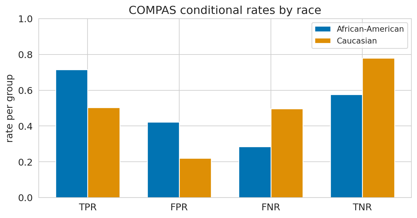
The headline numbers from the *ProPublica* analysis are here. Black defendants who did *not* go on to reoffend were flagged high risk at substantially higher rate than White defendants who did not. White defendants who *did* go on to reoffend were missed --- labeled low risk --- at substantially higher rate than Black defendants who did. The first comparison is the FPR row; the second is the FNR row. These are the gaps the *ProPublica* story was about.
A grouped bar chart makes the asymmetry visible:
```{python}
#| fig-cap: "COMPAS error rates by race. ProPublica's headline is the FPR pair: Black non-reoffenders were flagged high-risk at nearly twice the rate of White non-reoffenders. The mirror image appears in FNR."
fig, ax = plt.subplots(figsize=(7.5, 4))
metrics = ['TPR', 'FPR', 'FNR', 'TNR']
x = np.arange(len(metrics))
w = 0.35
palette = sns.color_palette('colorblind', 2)
for i, (race, row) in enumerate(rates.iterrows()):
    ax.bar(x + (i - 0.5) * w, row[metrics].values, w,
           label=race, color=palette[i])
ax.set_xticks(x)
ax.set_xticklabels(metrics)
ax.set_ylabel('rate per group')
ax.set_ylim(0, 1)
ax.set_title('COMPAS conditional rates by race')
ax.legend(loc='upper right', fontsize=10)
plt.tight_layout()
plt.show()
```
Reading the chart from left to right: COMPAS catches more of the people who do reoffend when they are Black (higher TPR), and falsely flags more of the people who do not when they are Black (higher FPR). The errors do not fall the same way on the two groups.
Equality of opportunity (equal TPR only) is the weaker condition. It asks the algorithm to identify the people who will reoffend at the same rate in each group, but does not constrain the false-positive rate. Equality of opportunity is the criterion to choose when the cost of a false negative is what you most want to equalize --- for example, in a screening tool for a treatable disease, you want to catch the same fraction of sick people in each group, and accept that the false-positive rate may differ.
## Predictive parity and calibration
So far the definitions have conditioned on the truth $y$ and asked whether the prediction was equally accurate. The next definitions condition on the *prediction* $\hat y$ and ask whether it meant the same thing across groups.
:::{.callout-important}
## Definition: predictive parity and calibration
A binary classifier satisfies *predictive parity* if its positive predictive value is equal across groups:
$$
P(y = 1 \mid \hat y = 1, a) \text{ does not depend on } a.
$$
A real-valued score $s$ satisfies *calibration within groups* if at each score level, the conditional outcome rate is the same across groups:
$$
P(y = 1 \mid s, a) \text{ does not depend on } a.
$$
The two are related: a score that is calibrated within groups satisfies predictive parity at every threshold used to binarize it.
:::
Predictive parity is the criterion that says "a score of 7 means the same thing about the future, regardless of which group the score is about." It is the criterion Northpointe invoked when responding to the *ProPublica* investigation.
Compute it on COMPAS:
```{python}
def ppv_npv(g):
    y = g['y'].values
    yh = g['y_hat'].values
    tp = ((y == 1) & (yh == 1)).sum()
    fp = ((y == 0) & (yh == 1)).sum()
    tn = ((y == 0) & (yh == 0)).sum()
    fn = ((y == 1) & (yh == 0)).sum()
    return pd.Series({
        'PPV': tp / (tp + fp) if tp + fp else np.nan,
        'NPV': tn / (tn + fn) if tn + fn else np.nan,
    })

pp = pd.DataFrame(
    {race: ppv_npv(g) for race, g in compas.groupby('race')}
).T.round(3)
print(pp)
```
The positive predictive value --- the share of people labeled high risk who actually went on to reoffend --- is close across groups, within a few percentage points. By the predictive-parity criterion, the score is approximately fair.
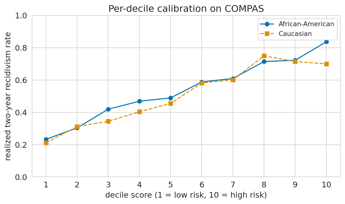
The full per-decile picture is the one Northpointe published: at each decile score, the realized two-year recidivism rate is close across groups.
```{python}
#| fig-cap: "Per-decile calibration on COMPAS by race. The two curves track each other across the score range: at any decile, the realized re-arrest rate is similar regardless of race. Northpointe pointed to this figure to argue the score is not biased."
calib = (compas.groupby(['decile_score', 'race'])['y']
               .mean().unstack())
fig, ax = plt.subplots(figsize=(7.5, 4.5))
palette = sns.color_palette('colorblind', 2)
linestyles = ['-', '--']
markers = ['o', 's']
for i, race in enumerate(calib.columns):
    ax.plot(calib.index, calib[race],
            marker=markers[i], linestyle=linestyles[i],
            color=palette[i], label=race)
ax.set_xlabel('decile score (1 = low risk, 10 = high risk)')
ax.set_ylabel('realized two-year recidivism rate')
ax.set_title('Per-decile calibration on COMPAS')
ax.set_ylim(0, 1)
ax.set_xticks(range(1, 11))
ax.legend(fontsize=10)
plt.tight_layout()
plt.show()
```
The two curves track each other across the score range. A defendant assigned decile 7 has approximately the same actual two-year recidivism rate regardless of race. The plot is the figure Northpointe pointed to in arguing the algorithm was not biased.
Both *ProPublica*'s claim (unequal FPR and FNR across groups) and Northpointe's claim (approximately equal PPV and per-decile calibration) are correct on the same data. The disagreement is not about the arithmetic. The disagreement is about which definition of fairness should govern.
## The impossibility: you cannot satisfy them all
The next result is the technical core of the chapter, and the reason the COMPAS dispute did not have a resolution. The intuition first: imagine two groups whose base rates differ. Calibration says the score has to mean the same thing in both groups --- the fraction of "high risk" labels that actually become positives has to match. Now pick anyone the model labeled positive in the higher-base-rate group; their re-arrest probability is fixed by calibration. The same labeled-positive in the lower-base-rate group has the *same* calibrated probability, but a *lower* prior odds of being a true positive. Bayes' rule then forces the false-positive rate (a likelihood ratio scaled by prior odds) to differ. Equalizing PPV across groups when base rates differ pulls the FPR and FNR apart. There is no clever algorithm that escapes the constraint.
:::{.callout-important}
## Result: impossibility of joint fairness
The result has two versions, on two different objects, both motivated by the COMPAS dispute.
**Binary classifier (Chouldechova 2017).**^[Chouldechova, A. (2017). "Fair prediction with disparate impact: A study of bias in recidivism prediction instruments." *Big Data*, 5(2), 153--163. arXiv:1703.00056.] If two groups have unequal base rates and a binary classifier has equal positive predictive value (PPV) across groups, then its false-positive and false-negative rates *cannot both* be equal across groups. The only escape is equal base rates or a classifier that never errs.
**Real-valued score (Kleinberg, Mullainathan, and Raghavan 2017).**^[Kleinberg, J., Mullainathan, S., & Raghavan, M. (2017). "Inherent Trade-Offs in the Fair Determination of Risk Scores." *Proceedings of the 8th Conference on Innovations in Theoretical Computer Science (ITCS 2017)*, paper 43. arXiv:1609.05807.] If two groups have unequal base rates, no non-trivial real-valued score can satisfy all three of: *calibration within groups* ($P(y=1 \mid s, a)$ does not depend on $a$), *balance for the positive class* (equal expected score on actual positives across groups), and *balance for the negative class* (equal expected score on actual negatives across groups). The same two escapes apply.
The two results are companion theorems on different objects. The binary version is the form most directly applicable to COMPAS (whose decile score becomes a binary detain/release decision via a threshold); the score version is the more general statement about probabilistic risk scores.
:::
On COMPAS, this constraint plays out exactly as the binary theorem predicts. PPV is approximately equal across groups (calibration roughly holds). Base rates differ by about 13 percentage points. The theorem then says the false-positive and false-negative rates *cannot both* be equal across groups --- at least one must differ. On COMPAS both do, and the direction is the one the algebra requires: the higher-base-rate group has the higher FPR; the lower-base-rate group has the higher FNR. A different algorithm cannot eliminate the constraint. Any algorithm can only choose which error to equalize at the cost of the others.
::: {.callout-note collapse="true"}
## Going deeper: the base-rate algebra
Chouldechova's derivation runs in two lines. Let $p = P(y=1)$ be the base rate, let $\text{TPR}$ and $\text{FPR}$ be the binary classifier's error rates, and let $\text{PPV}$ be its positive predictive value. By Bayes' rule,
$$
\text{PPV} \;=\; \frac{p \cdot \text{TPR}}{p \cdot \text{TPR} + (1 - p) \cdot \text{FPR}}.
$$
Solve for $\text{FPR}$ at fixed PPV and TPR:
$$
\text{FPR} \;=\; \frac{p}{1-p} \cdot \frac{1 - \text{PPV}}{\text{PPV}} \cdot \text{TPR}.
$$
If two groups share PPV (calibration) and TPR (equal opportunity), then $\text{FPR}$ scales with $p / (1 - p)$, which differs across groups whenever the base rate differs. The same algebra fixed in any two of $\{\text{PPV}, \text{TPR}, \text{FPR}\}$ forces the third to vary with $p$. The Kleinberg, Mullainathan, and Raghavan result extends the argument to real-valued scores rather than binary labels.
:::
What the impossibility does *not* tell you is which criterion to satisfy. The choice depends on the decision the model is supporting:
- A medical-screening tool with a cheap follow-up test: you probably want **equality of opportunity**. Catch the same fraction of sick people in each group, accept that the false-positive rate may differ.
- A bail decision with no easy reversal: you may want **equal false-positive rates**. At least make sure non-reoffenders are detained at the same rate, regardless of group.
- A credit-scoring model whose scores have to defend to a regulator that "650 means 650": **calibration within groups** is the natural target.
The choice depends on whose harm you are most committed to bounding, and on whose harm you are willing to redistribute to in order to bound it. Two careful analysts working with the same data --- a journalist and an engineer at the company that built the model, say --- can both do the arithmetic correctly and reach different conclusions about whether the model is fair, because they are operating with different answers to a values question that no algorithm decides for them.
## Counterfactual fairness, the causal bridge
The impossibility theorem ruled out *jointly* satisfying the four group-level criteria. It did not rule out a criterion of a different kind. Every metric so far has been a *group-level* one --- it conditions on the joint distribution of $(\hat y, y, a)$ and computes a marginal. Chapters 18 and 19 supplied the vocabulary --- causal models, directed acyclic graphs, counterfactuals --- for asking the fairness question at the *individual* level: would the model's prediction for *this person* change if their protected attribute were different, holding all the legitimate causes of the outcome fixed?
:::{.callout-important}
## Definition: counterfactual fairness
Write $A$ for the protected-attribute variable in the causal model and $a$, $a'$ for two possible values it could take. A predictor $\hat y$ is *counterfactually fair* if, for every individual whose factual attribute is $A = a$, the prediction we would get by intervening to set $A := a$ (the factual world) equals the prediction we would get by intervening to set $A := a'$ (the counterfactual world), with the intervention propagated through the structural causal model in both cases:
$$
\hat y_{A \leftarrow a}(x) \;=\; \hat y_{A \leftarrow a'}(x).
$$
The definition is due to Kusner, Loftus, Russell, and Silva.^[Kusner, M. J., Loftus, J. R., Russell, C., & Silva, R. (2017). "Counterfactual Fairness." *Advances in Neural Information Processing Systems 30 (NeurIPS 2017)*, pp. 4066--4076. arXiv:1703.06856.]
:::
Computing the counterfactual prediction means flipping $a$ and *propagating the flip through the causal model*: features the model treats as caused by $a$ (descendants of $a$ in the DAG) get updated under the flip; features the model treats as causes of $a$ (non-descendants) do not. Counterfactual fairness asks: under that propagation, would the prediction stay the same?
To make this concrete, return to the simulated structural causal model from the unawareness section. There, the proxy was generated as $\text{proxy} = 0.8\,z + 0.8\,a + \varepsilon$, so $a$ was a parent of $\text{proxy}$ in the DAG.
:::{.callout-tip}
## Think about it
The unaware model uses only the proxy as an input --- $a$ never appears. If we flip $a$ for every individual and re-derive their proxy (using the same noise the individual realized), how much do you think the unaware model's predictions move? Zero (since $a$ was never an input), small, or large?
:::
To compute the counterfactual prediction for an individual, we flip $a$ and *recompute* the proxy under the flipped $a$, holding the noise term $\varepsilon$ fixed at the value that individual realized:
```{python}
# Counterfactual world: flip a, recompute proxy with the same noise
a_cf       = 1 - a
proxy_cf   = 0.8 * z + 0.8 * a_cf + eps_proxy

sim_cf = sim.copy()
sim_cf['a']     = a_cf
sim_cf['proxy'] = proxy_cf

sim['p_unaware_cf'] = unaware.predict_proba(sim_cf[['proxy']])[:,1]
sim['delta']       = sim['p_unaware_cf'] - sim['p_unaware']

print('Mean absolute prediction change under counterfactual flip of a:')
print(np.abs(sim['delta']).mean().round(3))
print('\nPrediction change distribution:')
print(sim['delta'].describe().round(3))
```
The unaware model's prediction moves under the counterfactual flip. The proxy carried information about $a$, so changing $a$ changes the proxy, which changes the prediction. The unaware classifier is *not* counterfactually fair, even though by construction it never saw $a$.
Kusner et al. (2017) give a recipe for *constructing* a classifier that is counterfactually fair: identify, in the assumed structural causal model, the features that are descendants of $a$; refuse to use any of those features as inputs. The classifier may use non-descendants of $a$ freely. The cost is that you have to commit to a structural model --- a particular directed acyclic graph --- to say which features are descendants of $a$ and which are not. The resulting classifier is only as defensible as that graph is.
Two important caveats.
**For COMPAS, there is no credible structural causal model.** Race, in the US criminal-justice context, is entangled with neighborhood, schooling, policing intensity, family wealth, prior contacts with the system --- every feature COMPAS uses is plausibly a descendant of race in some structural-model sense, but the joint causal structure is contested rather than settled. We can compute the *statistical* fairness metrics from the four sections above on COMPAS. We cannot in good faith compute counterfactual fairness on COMPAS without specifying a structural causal model nobody would agree to.
**The counterfactual frame itself is contested.** A line of work by Issa Kohler-Hausmann and Lily Hu argues that the question "would the decision be the same if this person's race were different?" presupposes that race is a manipulable property of an individual that can be intervened on while holding other features fixed.^[Kohler-Hausmann, I. (2019). "Eddie Murphy and the Dangers of Counterfactual Causal Thinking About Detecting Racial Discrimination." *Northwestern University Law Review*, 113(5), 1163--1228. Hu, L., & Kohler-Hausmann, I. (2020). "What's Sex Got To Do With Fair Machine Learning?" *Proceedings of FAccT 2020*.] But race is also constitutive of features --- residence, schooling, peer networks, wealth --- that the counterfactual asks us to hold constant. Flipping race while fixing those features describes a person who does not exist. The implication is not that counterfactual fairness uses wrong arithmetic. It is that the entire research program of "what if this person were in the other group" rests on a contested foundation when the attribute being flipped is socially constructed.
::: {.callout-note collapse="true"}
## Going deeper: Plečko–Bareinboim and the Fairness Map
A unified causal-fairness framework due to Plečko and Bareinboim^[Plečko, D., & Bareinboim, E. (2024). "Causal Fairness Analysis: A Causal Toolkit for Fair Machine Learning." *Foundations and Trends in Machine Learning*, 17(3), 304--589. arXiv:2207.11385.] generalizes counterfactual fairness from a single yes/no criterion to a *decomposition*: the total observed disparity between groups is split into a direct effect of the protected attribute on the outcome, indirect effects through *legitimate* mediators (e.g., earned qualifications), and spurious effects through confounders. The decomposition organizes existing fairness definitions --- demographic parity, equalized odds, counterfactual fairness, path-specific fairness --- into a single *Fairness Map* hierarchy, with logical implications and incompatibilities made explicit. The R package `faircause` implements the decomposition; there is no first-party Python equivalent as of 2026. Plečko and Bareinboim is the natural graduate-level next step for this material.
:::
## Cases since COMPAS
The COMPAS dispute was not the only one. Three later cases, with primary-source documentation, show what the same lesson looks like in three other domains.
:::{.callout-note}
## Three cases since COMPAS
**Optum healthcare risk score (Obermeyer, Powers, Vogeli, and Mullainathan, *Science* 2019).**^[Obermeyer, Z., Powers, B., Vogeli, C., & Mullainathan, S. (2019). "Dissecting racial bias in an algorithm used to manage the health of populations." *Science*, 366(6464), 447--453. DOI: 10.1126/science.aax2342.] A widely deployed US population-health risk-stratification algorithm used by hospital systems to enroll patients into care-management programs. The label being predicted was *future healthcare cost*, not future illness. Because Black patients incurred less healthcare cost than equally-sick White patients --- due to barriers in access, lower trust, and other systemic factors --- the model's score systematically *understated* their morbidity: at any given algorithmic risk score, Black patients had more chronic conditions than White patients. Retraining on a morbidity-targeted label cut the chronic-condition disparity at the program-enrollment threshold by about 84%. The lesson is about *label design*, not metric choice.
**Dutch SyRI (Hague District Court, 5 February 2020).** A government cross-agency risk-scoring tool that combined tax, benefits, and employment records to flag individuals for welfare-fraud investigation, deployed primarily in low-income, immigrant-heavy neighborhoods. The Hague District Court ruled the SyRI law violated Article 8 of the European Convention on Human Rights for lack of transparency and discrimination risk, ordering the system halted. The first European court ruling to strike down a state algorithmic risk system on human-rights grounds.
**UK A-level grades (Ofqual, August 2020).** When 2020 A-level exams were cancelled, Ofqual's "standardisation" algorithm combined teacher predictions with historical school-level grade distributions to set grades. Roughly 39% of teacher-assigned grades were downgraded; students from large state schools (where the historical-distribution adjustment had more weight) were systematically downgraded relative to private-school students (whose smaller cohorts triggered fallback to teacher predictions). The algorithm was withdrawn four days after public release. The Ofqual chief executive resigned eight days after that.
:::
The pattern across these cases is not "the metric was wrong." It is that the choice of *what to measure* --- recidivism, cost, fraud probability, the cohort distribution to anchor a grade to --- and the *system in which the score becomes an action* turn out to be the load-bearing design decisions. The 2016--2017 fairness canon gives you the vocabulary to talk about those choices. The decisions themselves are human.
## What to do in practice
The chapter has spent most of its length on the technical question: what does fairness mean, and what does it imply about the choices a modeler can make. The practical question is broader. The published consensus in 2024--2026 has moved beyond "pick a metric and report it alongside accuracy" toward four ideas that work together rather than in competition.
The first is that fairness is a property of a *sociotechnical system*, not of a model. Selbst, boyd, Friedler, Venkatasubramanian, and Vertesi^[Selbst, A. D., boyd, d., Friedler, S. A., Venkatasubramanian, S., & Vertesi, J. (2019). "Fairness and Abstraction in Sociotechnical Systems." *Proceedings of the 2nd ACM Conference on Fairness, Accountability, and Transparency (FAT\* 2019)*, pp. 59--68.] identify five common abstraction "traps": modeling only the algorithm and not the institution it enters; assuming a fair model in one jurisdiction will be fair in another; assuming the formal definitions exhaust the meaning of fairness; ignoring how the algorithm itself reshapes the system; and assuming a technical fix exists at all. Metric choice is one input to a fairness assessment, not the assessment itself.
The second is that *auditing* has matured into a discipline. External and internal audits --- by journalists, by ombudspeople, by regulators, by independent contractors --- have produced the most credible findings of algorithmic discrimination on record. The EU AI Act, NYC Local Law 144, and the OMB M-24-10 directive (March 2024) all build mandatory audit obligations into the regulatory frame, so audits will continue to be produced whether or not the field's metric-of-the-month converges.
The third is that several design choices belong, at least in part, to the *affected community*. The label being predicted, the features that are admissible inputs, the threshold at which the score becomes an action, the recourse a person has after a bad prediction --- these are not metric choices and they are not engineering choices alone. A growing literature in HCI and public-sector design argues that these choices benefit from participation by the people the model will be applied to.
The fourth is that *compliance language* increasingly frames the technical work. Real fairness work-products in industry are now phrased as "Annex III high-risk Art. 10 data-governance obligation" rather than as research-paper claims. The compliance frame is unsentimental: it forces the organization to write down who is harmed and how, regardless of which metric is chosen.
If you have to do the technical work yourself, four open-source tools are in active maintenance and cover most of the practical landscape:
- **Fairlearn** (Microsoft, now independent open-source). `MetricFrame` disaggregates any scikit-learn metric by a sensitive attribute; `ThresholdOptimizer` post-processes a classifier to satisfy equalized odds, equality of opportunity, or demographic parity. The cleanest scikit-learn-style API; the first tool to reach for.
- **AIF360** (IBM / Linux Foundation AI). The broadest catalog of fairness metrics and mitigation algorithms. Heavier API; useful when you want to inspect the menu.
- **Aequitas** (DSAPP / University of Chicago). Built around the *bias-audit report* deliverable rather than retraining. Closest to what a municipal auditor would produce.
- **HolisticAI**. Newer; covers bias plus explainability, robustness, and other dimensions of trustworthy ML in one library --- closer in shape to what the EU AI Act's broader high-risk-system obligations actually require.
The course has argued throughout that taste --- the skill of recognizing what a model is and isn't telling you --- is the bottleneck. Fairness is the case where that argument is most pointed. The criteria are mathematically incompatible. The data does not pick between them. The choice belongs to whoever is responsible for the decision.
## Key takeaways
- **Unawareness isn't enough.** Removing the protected attribute from a model's inputs does not make its predictions independent of the attribute --- correlated features leak the signal back in.
- **Four group-fairness criteria, four different intuitions.** Demographic parity, equalized odds, equality of opportunity (a relaxation of equalized odds), and predictive parity each formalize a different intuition about what "fair" means. None is right in all settings.
- **The impossibility is real.** Kleinberg–Mullainathan–Raghavan (2017) and Chouldechova (2017): when group base rates differ, no non-trivial classifier can simultaneously satisfy predictive parity and equalized odds. The COMPAS dispute was an instance of this fact, not a mistake by either side.
- **Counterfactual fairness brings the causal vocabulary.** Kusner et al. (2017): would the prediction stay the same in a counterfactual world where the individual's protected attribute were different, propagated through the assumed structural causal model? It is the most demanding criterion and the one most dependent on a structural model the modeler has to commit to.
- **Fairness is a property of the system.** The consensus has moved beyond metric choice toward sociotechnical framing, audit obligations, participatory problem formulation, and regulatory compliance.
## Study guide
This chapter is enrichment material --- not on the final exam, no quiz problems. The recap below is for your own reading.
**Key ideas.**
- *Protected attribute* --- an attribute (race, sex, religion, age, disability, ...) on which a decision is legally forbidden to discriminate. Defined by statute.
- *Fairness through unawareness* --- withholding the protected attribute from the inputs. Insufficient on its own because correlated features leak the signal.
- *Demographic parity* --- equal positive prediction rate across groups; $\hat y \perp a$.
- *Equalized odds* --- equal TPR and equal FPR across groups; $\hat y \perp a \mid y$.
- *Equality of opportunity* --- equal TPR across groups (the weaker, qualified-group-focused version of equalized odds).
- *Predictive parity* --- equal PPV across groups; equivalently, *calibration within groups* at the score level.
- *Impossibility theorem* (Kleinberg–Mullainathan–Raghavan; Chouldechova) --- when base rates differ across groups, predictive parity and equalized odds cannot both hold for a non-trivial classifier.
- *Counterfactual fairness* (Kusner et al.) --- the prediction is unchanged when the protected attribute is flipped and the flip is propagated through the assumed structural causal model.
**Computational tools.**
- `sklearn.linear_model.LogisticRegression` --- fit a binary classifier; used here to demonstrate proxy leakage under unawareness.
- A *positive rate per group*, computed by `df.groupby(a)['y_hat'].mean()`.
- *Confusion-table rates per group* (TPR, FPR, PPV, ...), computed by group and shown as a small table or grouped bar chart.
- A *per-decile calibration plot* across groups --- realized outcome rate at each score level.
- The standard ProPublica COMPAS filter --- `days_b_screening_arrest` within ±30 days, `is_recid != -1`, ordinary charge degree, non-N/A score, two-race subset, decile-5 threshold for the binary classifier.
**Tooling for the field.**
- `fairlearn.metrics.MetricFrame` --- disaggregate any scikit-learn metric by a sensitive attribute.
- `fairlearn.postprocessing.ThresholdOptimizer` --- post-process to satisfy demographic parity, equalized odds, or equality of opportunity.
- `aif360`, `aequitas`, `holisticai` --- alternative libraries; broader catalogs, audit-report orientation, or trustworthy-ML integration.
**Further reading.** Barocas, Hardt, and Narayanan's open-access *Fairness and Machine Learning*^[Barocas, S., Hardt, M., & Narayanan, A. (2023). *Fairness and Machine Learning: Limitations and Opportunities*. MIT Press. Web version: <https://fairmlbook.org/>.] is the standard graduate text. The Plečko–Bareinboim monograph is the contemporary unified causal-fairness reference. The three cases in the *cases since COMPAS* callout each have primary-source documentation (court rulings, government inquiries, peer-reviewed articles) cited in the footnotes above.