---
title: "From the Mean to Simple Regression"
execute:
enabled: true
jupyter: python3
---
```{python}
import numpy as np
import pandas as pd
import matplotlib.pyplot as plt
import seaborn as sns
from sklearn.linear_model import LinearRegression
from sklearn.metrics import r2_score
import warnings
warnings.filterwarnings('ignore')
sns.set_style('whitegrid')
plt.rcParams['figure.figsize'] = (8, 5)
plt.rcParams['font.size'] = 12

# Load data
DATA_DIR = 'data'
```
## Am I pricing this right?
A friend just put their first Brooklyn listing on Airbnb and texts you: "Am I pricing this right?" Your first instinct: charge what typical listings charge — the average. But the average knows nothing about their listing. Their place has two bedrooms; bigger listings should cost more than smaller ones. Before you answer, you want a pricing model that reflects what you actually know about the listing.
This chapter builds such a model in two stages. Stage one ignores every feature and predicts a single number for every listing — the mean. Stage two lets the prediction respond to one feature, bedrooms, by fitting a line. Along the way, you will represent data as vectors, measure prediction error with norms, and discover that regression is really just a geometric projection.
Here is the roadmap:
1. **Vectors in data** — two ways to view a dataset, norms, and distances.
2. **Predicting with no features** — the mean as the best constant predictor.
3. **Predicting with one feature** — simple regression as a projection.
4. **How good is the fit?** — $R^2$, correlation, and the Pythagorean theorem.
5. **Regression to the mean** — why extreme observations revert toward the average.
```{python}
# Load the NYC Airbnb dataset
listings = pd.read_csv(f'{DATA_DIR}/airbnb/listings.csv', low_memory=False)

cols = ['id', 'name', 'price', 'bedrooms', 'bathrooms', 'beds',
        'room_type', 'neighbourhood_group_cleansed', 'accommodates',
        'number_of_reviews', 'review_scores_rating']
df = listings[cols].dropna(subset=['price', 'bedrooms', 'bathrooms']).copy()
df = df.rename(columns={'neighbourhood_group_cleansed': 'borough'})

# Price is already a clean integer column (no $ signs); filter to reasonable range
df['price'] = pd.to_numeric(df['price'], errors='coerce')
df = df[df['price'].between(10, 500)].reset_index(drop=True)
prices = df['price'].values

print(f"Working with {len(df):,} Airbnb listings")
df[['name', 'price', 'bedrooms', 'bathrooms', 'room_type', 'borough']].head()
```
# Vectors in data
## Two views of a dataset
A dataset is a table of numbers. There are two natural ways to see vectors in that table, and they answer different questions.
:::{.callout-important}
## Definition: Vector
A **vector** is an ordered list of numbers. In this course, a vector $v \in \mathbb{R}^d$ is a list of $d$ real numbers: $v = (v_1, v_2, \ldots, v_d)$. A **scalar** is a single number.
:::
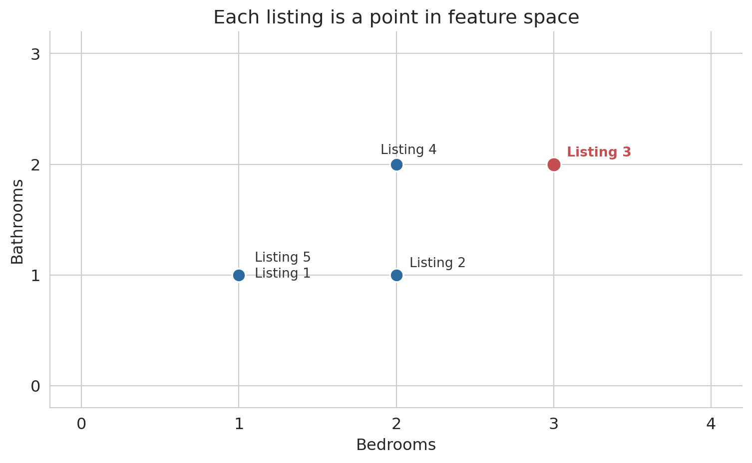
**Row view:** each listing is a point in feature space. A listing with 2 bedrooms, 1 bathroom, and a price of \$150 is the point $(2, 1, 150)$ in $\mathbb{R}^3$. Nearby points represent similar listings.
**Column view:** each feature is a vector across all $n$ listings. The "bedrooms" column is a vector in $\mathbb{R}^n$ — one entry per listing. Columns that trend together (bedrooms and price both increase for larger apartments) carry similar information.
Let's build intuition with a toy example: five listings with two features.
```{python}
# A tiny dataset: 5 Airbnb listings
bedrooms  = np.array([1, 2, 3, 2, 1])
bathrooms = np.array([1, 1, 2, 2, 1])
toy_price = np.array([100, 150, 250, 200, 120])

print("Row view — each listing is a point in R^2:")
for i in range(5):
    print(f"  Listing {i+1}: ({bedrooms[i]}, {bathrooms[i]})")
print()
print(f"Column view — bedrooms is a vector in R^5: {bedrooms}")
print(f"Column view — bathrooms is a vector in R^5: {bathrooms}")
```
## Rows as points
Each listing occupies a position in feature space. Listings with similar features sit close together; dissimilar listings sit far apart.
```{python}
fig, ax = plt.subplots(figsize=(8, 5))

point_color = '#2d6a9f'
highlight_color = '#c44e52'

ax.scatter(bedrooms, bathrooms, s=100, color=point_color,
           edgecolors='white', linewidths=1.2, zorder=5)

# Highlight Listing 3
ax.scatter([bedrooms[2]], [bathrooms[2]], s=120, color=highlight_color,
           edgecolors='white', linewidths=1.2, zorder=6)

# Labels
offsets = [(12, -2), (10, 6), (10, 6), (-12, 8), (12, 10)]
for i, off in enumerate(offsets):
    color = highlight_color if i == 2 else '#333333'
    weight = 'semibold' if i == 2 else 'normal'
    ax.annotate(f'Listing {i+1}', (bedrooms[i], bathrooms[i]),
                fontsize=10, color=color, fontweight=weight,
                xytext=off, textcoords='offset points')

ax.set_xlabel('Bedrooms')
ax.set_ylabel('Bathrooms')
ax.set_title('Each listing is a point in feature space')
ax.set_xlim(-0.2, 4.2)
ax.set_ylim(-0.2, 3.2)
ax.set_xticks([0, 1, 2, 3, 4])
ax.set_yticks([0, 1, 2, 3])
for spine in ['top', 'right']:
    ax.spines[spine].set_visible(False)
plt.tight_layout()
plt.show()
```
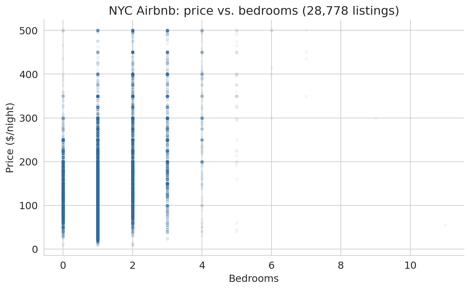
Scaling up from five listings to 28,778, the row view becomes a scatter plot of every listing positioned by two features. The figure below plots price against bedrooms for the full NYC dataset. Each gray dot is one listing; larger apartments drift toward higher prices.
```{python}
fig, ax = plt.subplots(figsize=(8, 5))
ax.scatter(df['bedrooms'], prices, alpha=0.04, s=10, color='#2d6a9f')
ax.set_xlabel('Bedrooms')
ax.set_ylabel('Price ($/night)')
ax.set_title(f'NYC Airbnb: price vs. bedrooms ({len(df):,} listings)')
for spine in ['top', 'right']:
    ax.spines[spine].set_visible(False)
plt.tight_layout()
plt.show()
```
The upward drift is the pattern a linear model will try to capture. Hold on to the picture — we will return to it repeatedly as the chapter develops.
## Difference vector and distance
How different are two listings? Subtract their feature vectors entry by entry to get a **difference vector**.
```{python}
listing_1 = np.array([bedrooms[0], bathrooms[0]])  # (1, 1)
listing_3 = np.array([bedrooms[2], bathrooms[2]])  # (3, 2)
diff = listing_3 - listing_1

print(f"Listing 1: {listing_1}")
print(f"Listing 3: {listing_3}")
print(f"Difference: {listing_3} - {listing_1} = {diff}")
print(f"\nListing 3 has {diff[0]} more bedrooms and {diff[1]} more bathroom.")
```
The difference vector tells us *how* two listings differ, but the result is still two numbers. To collapse the difference into a single number that measures "how far apart," we need the length of the difference vector.
:::{.callout-important}
## Definition: Norm
The **norm** (or **length**) of a vector $v$ is
$$\|v\| = \sqrt{\sum_{i=1}^n v_i^2}$$
The norm generalizes the Pythagorean theorem to any number of dimensions. In code: `np.linalg.norm(v)`.
:::
The **distance** between two vectors is the norm of their difference: $d(u, v) = \|u - v\|$.
```{python}
dist = np.linalg.norm(diff)
print(f"Difference vector: {diff}")
print(f"Distance = ||diff|| = sqrt({diff[0]}² + {diff[1]}²) = {dist:.2f}")
```
## Columns as vectors in $\mathbb{R}^n$
Now flip your perspective. Instead of one listing as a point in feature space, look at one *feature* as a vector across all listings. The price column is a vector in $\mathbb{R}^n$ — one entry per listing. So is the bedrooms column.
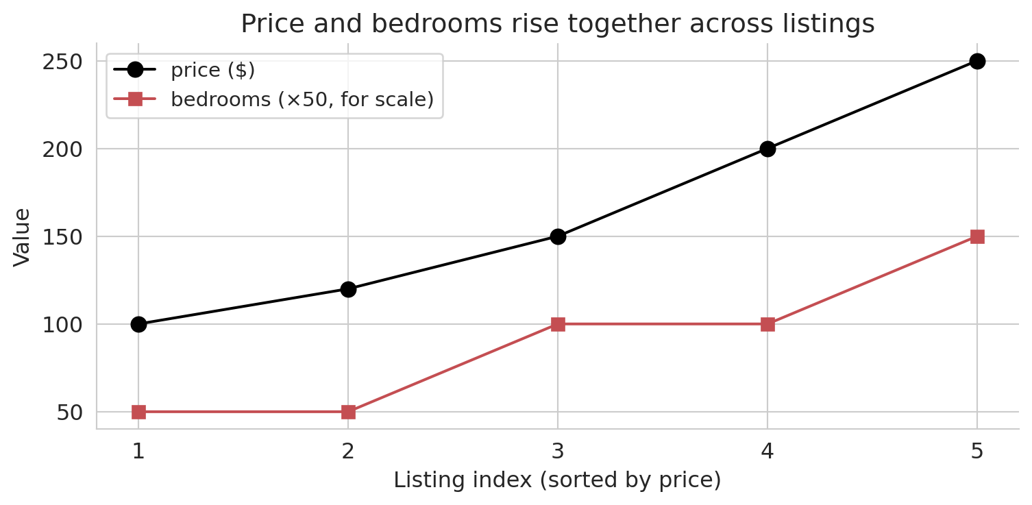
We can't plot these vectors in $\mathbb{R}^n$: any picture we make is in $\mathbb{R}^2$. Instead, an **index plot** can visualize these high-dimensional vectors. Each dot represents one listing, plotted by its index (horizontal) and feature value (vertical). The index plot below sorts the five toy listings by price and overlays bedrooms on the same axis.
```{python}
# Sort listings by price to reveal structure
sort_idx = np.argsort(toy_price)
sorted_price = toy_price[sort_idx]
sorted_beds = bedrooms[sort_idx]

fig, ax = plt.subplots(figsize=(8, 4))
indices = np.arange(len(toy_price))

ax.plot(indices, sorted_price, 'ko-', ms=8, lw=1.5, label='price ($)', zorder=5)
ax.plot(indices, sorted_beds * 50, 's-', color='#c44e52', ms=7, lw=1.5,
        label='bedrooms (×50, for scale)', zorder=4)

ax.set_xlabel('Listing index (sorted by price)')
ax.set_ylabel('Value')
ax.set_title('Price and bedrooms rise together across listings')
ax.set_xticks(indices)
ax.set_xticklabels([f'{i+1}' for i in range(len(indices))])
ax.legend(fontsize=11)
for spine in ['top', 'right']:
    ax.spines[spine].set_visible(False)
plt.tight_layout()
plt.show()
```
Price and bedrooms rise together: the two columns are correlated. In this chapter, correlation gets a geometric meaning — two correlated columns, viewed as vectors in $\mathbb{R}^n$, point in similar directions. The tool that quantifies "similar direction" is the **inner product**.
:::{.callout-important}
## Definition: Inner product (dot product)
The **inner product** of two vectors $u, v \in \mathbb{R}^n$ is
$$u^T v = \sum_{i=1}^n u_i v_i$$
A positive inner product means the vectors tend to point in the same direction; a negative value means opposite directions; zero means the vectors are **orthogonal** (perpendicular).
:::
The formula matches the index plot exactly. Multiply price and bedrooms entry by entry, then add. When both vectors are large at the same listings, every product is large and the sum piles up — a big positive inner product signals a shared direction in $\mathbb{R}^n$.
```{python}
# Inner product between price and bedrooms (on the toy data)
dot_price_beds = np.dot(toy_price, bedrooms)
print(f"price · bedrooms = {dot_price_beds}")
print(f"Both vectors trend upward → large positive inner product")
```
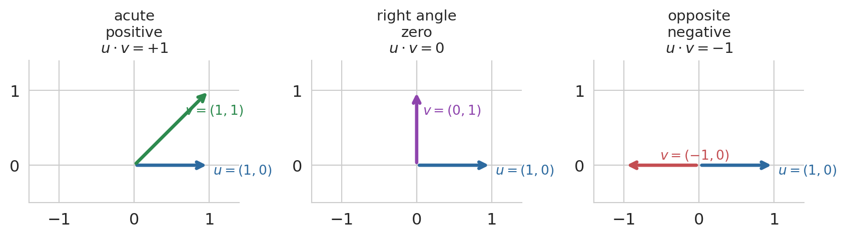
A two-dimensional picture builds the intuition for the sign. Pin $u = (1, 0)$ pointing along the x-axis, and sweep a second vector $v$ through three positions: leaning into the same half-plane (acute angle, positive dot product), straight up (right angle, zero), and pointing the opposite way (obtuse angle, negative). The sign of the inner product tracks the angle between the vectors.
```{python}
#| code-fold: true
fig, axes = plt.subplots(1, 3, figsize=(9, 3.2))

cases = [
    (np.array([1, 1]),  '$v = (1, 1)$',  '$u \\cdot v = +1$',  '#2d8a4e', 'acute\npositive'),
    (np.array([0, 1]),  '$v = (0, 1)$',  '$u \\cdot v = 0$',   '#8e44ad', 'right angle\nzero'),
    (np.array([-1, 0]), '$v = (-1, 0)$', '$u \\cdot v = -1$',  '#c44e52', 'opposite\nnegative'),
]
u = np.array([1, 0])

for ax, (v, vlab, dot_lab, col, tag) in zip(axes, cases):
    ax.annotate('', xy=u, xytext=(0, 0),
                arrowprops=dict(arrowstyle='->', color='#2d6a9f', lw=2.5))
    ax.text(u[0] + 0.05, u[1] - 0.12, '$u = (1, 0)$', fontsize=10, color='#2d6a9f')
    ax.annotate('', xy=v, xytext=(0, 0),
                arrowprops=dict(arrowstyle='->', color=col, lw=2.5))
    ax.text(v[0] * 0.6 + 0.08, v[1] * 0.6 + 0.08, vlab, fontsize=10, color=col)
    ax.set_title(f'{tag}\n{dot_lab}', fontsize=11)
    ax.set_xlim(-1.4, 1.4)
    ax.set_ylim(-0.5, 1.4)
    ax.set_aspect('equal')
    ax.axhline(0, color='#cccccc', lw=0.8, zorder=0)
    ax.axvline(0, color='#cccccc', lw=0.8, zorder=0)
    for spine in ['top', 'right']:
        ax.spines[spine].set_visible(False)
    ax.set_xticks([-1, 0, 1])
    ax.set_yticks([0, 1])

plt.tight_layout()
plt.show()
```
:::{.callout-important}
## Definition: Orthogonal
Two vectors $u$ and $v$ are **orthogonal** if $u^T v = 0$. Orthogonal vectors are perpendicular — they share no common direction.
:::
The raw inner product has a shortcoming: it mixes direction with magnitude. Scale the price column from dollars to cents and the inner product grows 100-fold, even though the geometric relationship is unchanged. To isolate direction, center each vector (subtract its mean so deviations from average are on equal footing) and then divide by norms. The result is the **correlation coefficient** you already know from probability.
:::{.callout-important}
## Definition: Correlation
The **Pearson correlation coefficient** between two vectors $u, v \in \mathbb{R}^n$ is the inner product of their centered, length-normalized versions:
$$r(u, v) = \frac{(u - \bar{u})^T (v - \bar{v})}{\|u - \bar{u}\| \; \|v - \bar{v}\|}$$
where $\bar{u} = \frac{1}{n}\sum_i u_i$ is the mean of $u$ (similarly for $v$). The value of $r$ is always between $-1$ and $+1$:
- $r = +1$: the centered vectors point in the same direction (perfect positive linear association).
- $r = -1$: they point in opposite directions (perfect negative linear association).
- $r = 0$: the centered vectors are orthogonal — no linear information.
Correlation is unitless: scaling either column by a positive constant leaves $r$ unchanged.
:::
```{python}
# Correlation between price and bedrooms on the full dataset
r_price_beds = df['price'].corr(df['bedrooms'])
print(f"r(price, bedrooms) = {r_price_beds:.4f}")
print("Positive and moderate — prices and bedrooms move together, "
      "but bedrooms is far from the whole story.")
```
Correlation and orthogonality are the two endpoints we will use throughout the chapter: correlated columns contribute to prediction, orthogonal residuals signal that no further correlation remains to exploit.
# Predicting with no features
## The simplest predictor: a constant
Before using any features at all, consider the simplest possible prediction: guess the same number $c$ for every listing.
How bad is this guess?
The **residual error** for listing $i$ is $\epsilon_i = y_i - c$.
Define the vector of all 1's, $\mathbf{1}$.
In vector notation, our predictions are $c \mathbf{1}$,
and the residual vector $\epsilon = y - c\mathbf{1}$ collects all the individual errors.
We can see these errors on an index plot.
Black dots are the actual prices, the green horizontal line is a constant prediction $\hat{y}$, and the vertical segments are the residuals.
```{python}
# Visualize residuals
y_bar = toy_price.mean()

fig, ax = plt.subplots(figsize=(8, 4))
indices = np.arange(len(toy_price))
ax.scatter(indices, toy_price, color='black', s=60, zorder=5, label='actual price $y_i$')
ax.axhline(y_bar, color='#2d8a4e', lw=2.5, ls='--', label=f'mean $\\bar{{y}}$ = {y_bar:.0f}')

for i in range(len(toy_price)):
    ax.plot([i, i], [toy_price[i], y_bar], color='#c44e52', lw=1.5, alpha=0.7)

ax.set_xlabel('Listing index')
ax.set_ylabel('Price ($)')
ax.set_title('Residuals from predicting a constant')
ax.set_xticks(indices)
ax.set_xticklabels([f'{i+1}' for i in range(len(indices))])
ax.legend(fontsize=11)
for spine in ['top', 'right']:
    ax.spines[spine].set_visible(False)
plt.tight_layout()
plt.show()

residuals = toy_price - y_bar
print(f"Residual vector: {residuals}")
```
## The best constant guess
What single number should you guess?
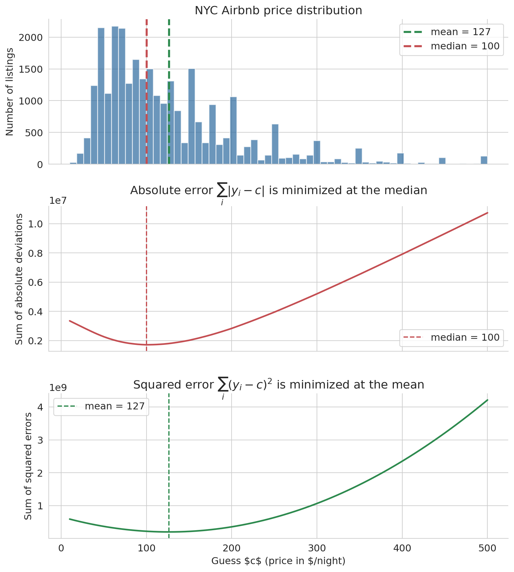
The answer depends on how you measure error. Two natural error measures are the sum of absolute deviations $\sum_i |y_i - c|$ and the sum of squared errors $\sum_i (y_i - c)^2$. The figure below computes both losses on the full NYC Airbnb price column for a sweep of candidate constants $c$.
```{python}
# Stacked view: real price distribution on top, then the two loss curves
# evaluated on the full price column.
c_values = np.linspace(10, 500, 400)
abs_errors = np.array([np.sum(np.abs(prices - c)) for c in c_values])
sq_errors  = np.array([np.sum((prices - c)**2)    for c in c_values])

mean_price = prices.mean()
median_price = np.median(prices)

fig, axes = plt.subplots(3, 1, figsize=(9, 10), sharex=True)

# Row 1: histogram of real prices with mean and median marked
axes[0].hist(prices, bins=60, color='#2d6a9f', alpha=0.7, edgecolor='white')
axes[0].axvline(mean_price, color='#2d8a4e', lw=2.5, ls='--',
                label=f'mean = {mean_price:.0f}')
axes[0].axvline(median_price, color='#c44e52', lw=2.5, ls='--',
                label=f'median = {median_price:.0f}')
axes[0].set_ylabel('Number of listings')
axes[0].set_title('NYC Airbnb price distribution')
axes[0].legend()

# Row 2: sum of absolute deviations — V-shape, min at the median
axes[1].plot(c_values, abs_errors, lw=2, color='#c44e52')
axes[1].axvline(median_price, color='#c44e52', ls='--', lw=1.5,
                label=f'median = {median_price:.0f}')
axes[1].set_ylabel('Sum of absolute deviations')
axes[1].set_title(r'Absolute error $\sum_i |y_i - c|$ is minimized at the median')
axes[1].legend()

# Row 3: sum of squared errors — parabola, min at the mean
axes[2].plot(c_values, sq_errors, lw=2, color='#2d8a4e')
axes[2].axvline(mean_price, color='#2d8a4e', ls='--', lw=1.5,
                label=f'mean = {mean_price:.0f}')
axes[2].set_xlabel(r'Guess $c$ (price in $/night)')
axes[2].set_ylabel('Sum of squared errors')
axes[2].set_title(r'Squared error $\sum_i (y_i - c)^2$ is minimized at the mean')
axes[2].legend()

for ax in axes:
    for spine in ['top', 'right']:
        ax.spines[spine].set_visible(False)
plt.tight_layout()
plt.show()
```
Minimizing absolute error gives the **median**. Minimizing squared error gives the **mean**. The shared x-axis makes the alignment visual: the V-shape bottoms out at the median, the parabola bottoms out at the mean, and both picks sit inside the bulk of the distribution above.
:::{.callout-tip}
## Think about it
Why does the choice of loss function pick out a different summary? Squared error favors the mean, absolute error favors the median. Before reading the proof below, ask yourself: what happens to the derivative of $(y_i - c)^2$ as $c$ moves through the data, and why does that force a balance at $\bar{y}$?
:::
We verify the squared-error result with a one-line calculus proof.
**Why squared error gives the mean.** We want the constant $c$ that minimizes $\sum_i (y_i - c)^2$. Take the derivative with respect to $c$ and set it to zero:
$$\frac{d}{dc} \sum_{i=1}^n (y_i - c)^2 = -2\sum_{i=1}^n (y_i - c) = 0 \quad \Longrightarrow \quad c = \frac{1}{n}\sum_{i=1}^n y_i = \bar{y}$$
The optimal constant prediction under squared error is the sample mean $\bar{y}$. The absolute-error result takes more work: $|y_i - c|$ is not differentiable at $c = y_i$, so no calculus proof applies. The median emerges from a discrete balancing argument — when half the data points are above and half below, there's no benefit to changing $c$.
:::{.callout-tip}
## Think about it
The squared-error curve is a smooth parabola; the absolute-error curve has a sharp V. What does the shape of each curve tell you about sensitivity to small changes in your guess? If you shift $c$ by one dollar near the optimum, which loss punishes you more — absolute or squared?
:::
## Notation
Let's establish the notation we will use throughout the rest of the book. Standard statistics notation puts a hat $\hat y$ on any quantity estimated from data, pronounced "y hat".
:::{.callout-important}
## Definition: Regression notation
- $y = (y_1, \ldots, y_n)$ — the **response** vector (actual prices)
- $\hat{y} = (\hat{y}_1, \ldots, \hat{y}_n)$ — the **prediction** vector
- $\bar{y} = \frac{1}{n}\sum_i y_i$ — the **sample mean** of $y$
- $\epsilon = y - \hat{y}$ — the **residual** vector (prediction errors)
- $\beta_0$ — the **intercept** (the constant term in the model)
:::
For the constant model, the prediction $\hat{y}_i = \beta_0$ for all $i$, and the best choice is $\hat{\beta}_0 = \bar{y}$, the mean of the responses.
## Residuals sum to zero
When $\hat{y} = \bar{y}$ for every listing, the residuals satisfy a simple but important identity:
$$\sum_{i=1}^n \epsilon_i = \sum_{i=1}^n (y_i - \bar{y}) = n\bar{y} - n\bar{y} = 0$$
In vector notation, $\mathbf{1}^T \epsilon = 0$, where $\mathbf{1}$ is the vector of all ones. The positive and negative errors cancel exactly. This identity will reappear — and generalize — when we move to regression.
```{python}
# Verify: residuals from the mean sum to zero
y_bar_full = prices.mean()
residuals_mean = prices - y_bar_full

print(f"Mean price: ${y_bar_full:.2f}")
print(f"Sum of residuals: {np.sum(residuals_mean):.6f}  (≈ 0)")
```
## The mean ignores features
The mean is optimal among constant predictions, but a constant prediction ignores everything we know about each listing. The scatter plot below shows price versus bedrooms with a horizontal line at $\bar{y}$. The mean captures the overall level but misses the upward trend — larger listings cost more.
```{python}
fig, ax = plt.subplots(figsize=(8, 5))
ax.scatter(df['bedrooms'], prices, alpha=0.04, s=10, color='#aaaaaa')
ax.axhline(y_bar_full, color='#2d8a4e', lw=2.5, ls='--',
           label=f'constant prediction $\\bar{{y}}$ = ${y_bar_full:.0f}')
ax.set_xlabel('Bedrooms')
ax.set_ylabel('Price ($/night)')
ax.set_title('The mean cannot capture the bedrooms-price pattern')
ax.legend(fontsize=11, loc='upper left')
for spine in ['top', 'right']:
    ax.spines[spine].set_visible(False)
plt.tight_layout()
plt.show()
```
# Predicting with one feature
## From constant to linear
The mean ignores bedrooms entirely. Can we do better by letting the prediction vary with bedrooms? The simplest way: a straight line.
$$\hat{y}_i = \beta_0 + \beta_1 \, x_i$$
where $x_i$ is the number of bedrooms for listing $i$. The prediction $\hat{y}$ is a **linear combination** of two column vectors: the ones vector $\mathbf{1}$ (scaled by $\beta_0$) and the bedrooms vector $x$ (scaled by $\beta_1$).
:::{.callout-important}
## Definition: Linear combination
A **linear combination** of vectors $v_1, v_2$ is any expression $\beta_1 v_1 + \beta_2 v_2$, where $\beta_1, \beta_2$ are scalars (plain numbers). The prediction $\hat{y} = \beta_0 \mathbf{1} + \beta_1 x$ is a linear combination of two column vectors.
:::
## The span: all reachable predictions
Different choices of $(\beta_0, \beta_1)$ produce different prediction vectors. The **span** of $\mathbf{1}$ and $x$ is the set of *all* prediction vectors you can reach by varying the weights.
:::{.callout-important}
## Definition: Span
The **span** of vectors $v_1, v_2$ is the set of all their linear combinations:
$$\text{span}(v_1, v_2) = \{\beta_1 v_1 + \beta_2 v_2 : \beta_1, \beta_2 \in \mathbb{R}\}$$
For a linear model $\hat{y} = \beta_0 \mathbf{1} + \beta_1 x$, the span is the set of all possible predictions — every line you could draw through the scatter plot.
:::
```{python}
# Fit the least-squares line once; we'll use it as one of the candidates
# in the two visualizations below.
model = LinearRegression().fit(df[['bedrooms']], prices)
b0, b1 = model.intercept_, model.coef_[0]
print(f"Least-squares fit: ŷ = {b0:.0f} + {b1:.0f} × bedrooms")
```
Each $(\beta_0, \beta_1)$ traces a different line on the bedrooms-vs-price scatter plot. The plot below overlays four candidates.
:::{.callout-tip}
## Think about it
Look at the four candidate lines below. Which one do you think minimizes the total squared error — and what criterion is your eye implicitly using to decide? "Passes through the middle of the cloud" is a starting point; try to make the criterion precise enough that you could compute it.
:::
```{python}
fig, ax = plt.subplots(figsize=(8, 5))
ax.scatter(df['bedrooms'], prices, alpha=0.04, s=10, color='#cccccc')

x_line = np.linspace(0, 6, 100)
candidates = [
    (50,   30, '#e74c3c', f'low intercept: ŷ = 50 + 30x'),
    (150,  30, '#3498db', f'high intercept: ŷ = 150 + 30x'),
    (100, -10, '#8e44ad', f'wrong sign: ŷ = 100 − 10x'),
    (b0,   b1, '#2d8a4e', f'least squares: ŷ = {b0:.0f} + {b1:.0f}x'),
]

for c0, c1, color, label in candidates:
    ax.plot(x_line, c0 + c1 * x_line, lw=2, color=color, label=label, alpha=0.85)

ax.set_xlabel('Bedrooms')
ax.set_ylabel('Price ($/night)')
ax.set_title('Many lines are possible — which is best?')
ax.set_ylim(0, 400)
ax.legend(fontsize=10)
for spine in ['top', 'right']:
    ax.spines[spine].set_visible(False)
plt.tight_layout()
plt.show()
```
The red and blue lines share the same slope but disagree on where the line should start. The purple line slopes the wrong way — more bedrooms should raise the price, not lower it. The green line is the one scikit-learn will find in a moment; for now it is just another candidate.
### How big is the span, really?
The scatter plot above is misleading in one important way. It makes the span *look* enormous: any slope, any intercept, any line you want. Every choice of $(\beta_0, \beta_1)$ gives a new line, and there are infinitely many of them. From this 2D picture, it looks like you can reach anything.
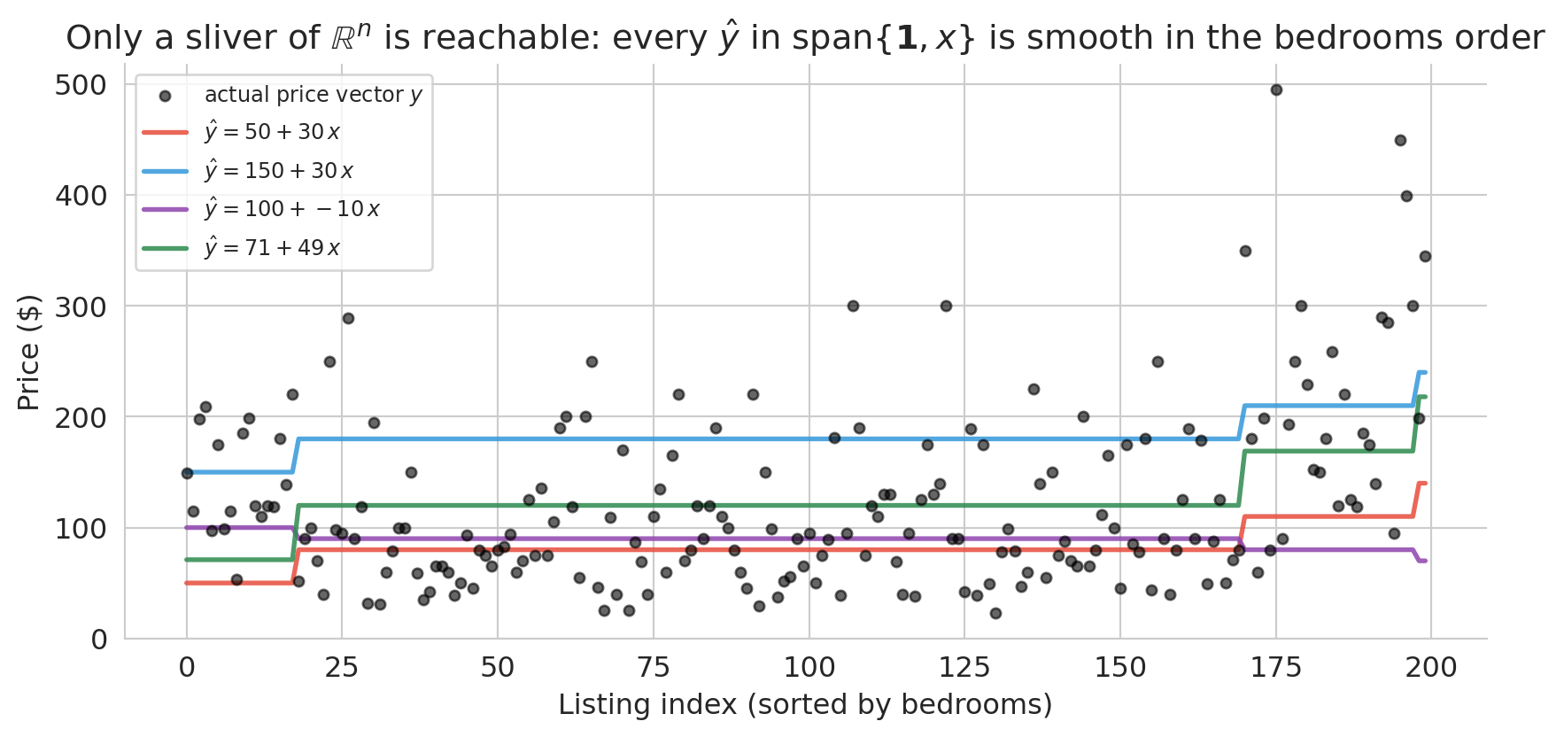
That picture hides the real geometry. The actual prediction vector $\hat{y}$ has one coordinate per listing — it lives in $\mathbb{R}^n$, where $n$ is the number of listings (here, close to 30,000). The span of $\{\mathbf{1}, x\}$ is a two-dimensional plane inside that vast space — a sliver. To see the constraint, switch from the scatter view to the index view, where all $n$ coordinates appear at once.
```{python}
#| code-fold: true
# Span is only 2D: on the index plot you can see that tuning (β₀, β₁)
# produces very smooth prediction vectors — nothing like the noisy real prices.
rng = np.random.default_rng(0)
sample_idx = rng.choice(len(df), size=200, replace=False)
beds_sample = df['bedrooms'].values[sample_idx]
price_sample = prices[sample_idx]
order = np.argsort(beds_sample)
beds_sorted_s = beds_sample[order]
price_sorted_s = price_sample[order]

fig, ax = plt.subplots(figsize=(9, 4.5))
idx = np.arange(len(beds_sorted_s))

# Real price vector: noisy, zigzags even after sorting
ax.scatter(idx, price_sorted_s, s=18, color='black', alpha=0.6,
           label='actual price vector $y$', zorder=3)

# The same four candidates from the scatter plot above
candidates_span = [(50, 30, '#e74c3c'),
                   (150, 30, '#3498db'),
                   (100, -10, '#8e44ad'),
                   (round(b0), round(b1), '#2d8a4e')]
for c0, c1, color in candidates_span:
    pred = c0 + c1 * beds_sorted_s
    ax.plot(idx, pred, color=color, lw=2, alpha=0.85,
            label=f'$\\hat y = {c0:.0f} + {c1:.0f}\\,x$')

ax.set_xlabel('Listing index (sorted by bedrooms)')
ax.set_ylabel('Price ($)')
ax.set_title('Only a sliver of $\\mathbb{R}^n$ is reachable: every $\\hat{y}$ '
             'in span$\\{\\mathbf{1}, x\\}$ is smooth in the bedrooms order')
ax.legend(fontsize=9, loc='upper left')
for spine in ['top', 'right']:
    ax.spines[spine].set_visible(False)
plt.tight_layout()
plt.show()
```
The black dots are a 200-listing sample of the actual prices, sorted by bedrooms. They zigzag across the plot — a 1-bedroom listing can cost anywhere from \$30 to \$400, because bedrooms is not the only thing that determines price. The colored curves are the *same four candidates* from the scatter plot above, now drawn on the index view. Each one collapses to a piecewise-constant staircase: listings with the same bedroom count get the same prediction, so tuning $(\beta_0, \beta_1)$ only controls the height and slope of the steps. No matter how we choose the weights, the prediction vector cannot zigzag the way the real prices do.
That is the real geometry. The span is a two-parameter sliver of $\mathbb{R}^n$, not the whole space. Most vectors in $\mathbb{R}^n$ cannot be produced at all. Our job is not to reach the true price vector — we cannot — but to find the closest point in the sliver to $y$. To *decide* which candidate is closest we need a principled criterion, and the right criterion turns out to be geometric.
## The geometric view: projection
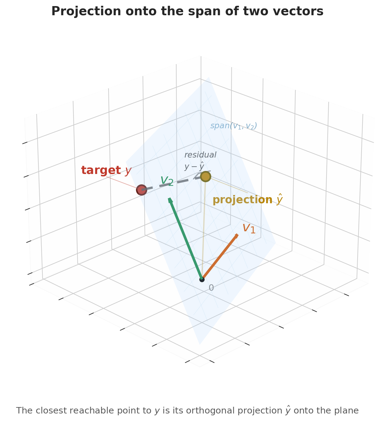
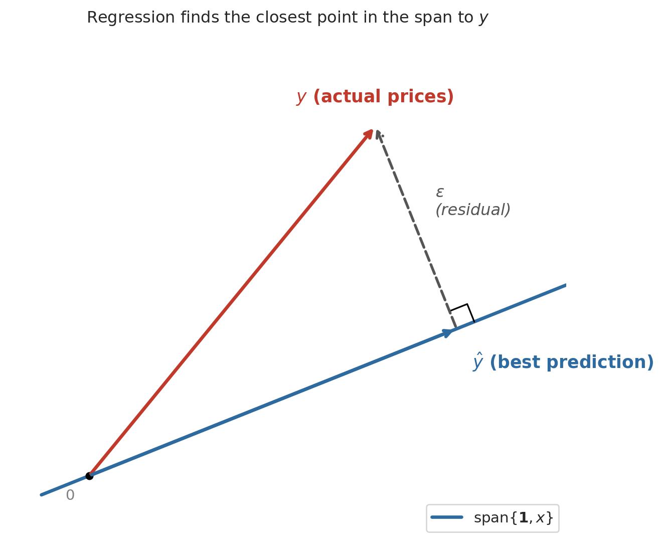
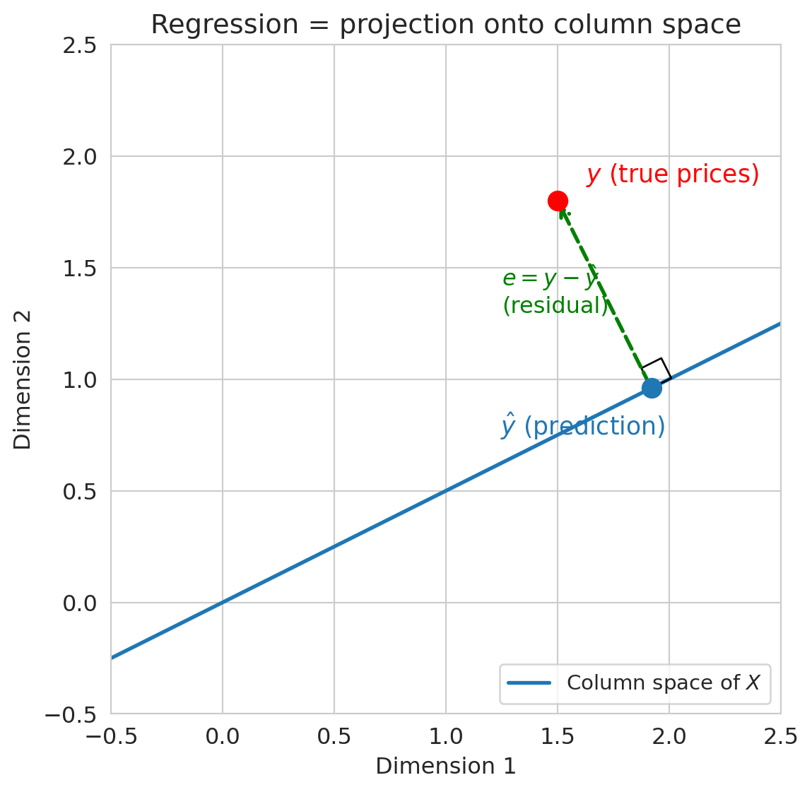
Here is the key geometric insight. Switch to the column view. With $n$ listings, the price vector $y$, the ones vector $\mathbf{1}$, and the bedrooms vector $x$ all live in $\mathbb{R}^n$ — one coordinate per listing. Picture the span of $\mathbf{1}$ and $x$ as a flat two-dimensional plane floating inside that high-dimensional space. Every possible regression line — every choice of $(\beta_0, \beta_1)$ — is a single point on that plane. The actual price vector $y$ is a point off the plane, because no single line fits every listing perfectly.
The best prediction $\hat{y}$ is the point in the plane closest to $y$ — the foot of the perpendicular dropped from $y$ onto the plane. Geometry calls the closest point the **orthogonal projection**, and it is the point where the residual $\epsilon = y - \hat{y}$ is perpendicular to the plane itself.
```{python}
#| code-fold: true
# Cartoon: y projected onto span{1, x}
fig, ax = plt.subplots(figsize=(7, 6))

# The plane (shown as a line in 2D)
t = np.linspace(-0.3, 3.0, 100)
ax.plot(t, 0.4 * t, color='#2d6a9f', lw=2.5, label='span{$\\mathbf{1}, x$}')

y_pt = np.array([1.8, 2.2])
d = np.array([1, 0.4])
d_unit = d / np.linalg.norm(d)
yhat_pt = np.dot(y_pt, d_unit) * d_unit
e_vec = y_pt - yhat_pt

# Vectors
ax.annotate('', xy=y_pt, xytext=(0, 0),
            arrowprops=dict(arrowstyle='->', color='#c0392b', lw=2.5))
ax.text(y_pt[0] - 0.5, y_pt[1] + 0.15, '$y$ (actual prices)',
        fontsize=13, color='#c0392b', fontweight='bold')

ax.annotate('', xy=yhat_pt, xytext=(0, 0),
            arrowprops=dict(arrowstyle='->', color='#2d6a9f', lw=2.5))
ax.text(yhat_pt[0] + 0.1, yhat_pt[1] - 0.25, '$\\hat{y}$ (best prediction)',
        fontsize=13, color='#2d6a9f', fontweight='bold')

ax.annotate('', xy=y_pt, xytext=yhat_pt,
            arrowprops=dict(arrowstyle='->', color='#555555', lw=2, ls='--'))
mid = (y_pt + yhat_pt) / 2
ax.text(mid[0] + 0.12, mid[1] + 0.08, '$\\epsilon$\n(residual)',
        fontsize=12, color='#555555', style='italic')

# Right angle
sz = 0.12
p_dir = d_unit
r_dir = e_vec / np.linalg.norm(e_vec)
sq = np.array([yhat_pt + sz*p_dir,
               yhat_pt + sz*p_dir + sz*r_dir,
               yhat_pt + sz*r_dir])
ax.plot(sq[:, 0], sq[:, 1], 'k-', lw=1.2)

ax.plot(0, 0, 'ko', ms=5)
ax.text(-0.15, -0.15, '$0$', fontsize=11, color='gray')

ax.set_xlim(-0.5, 3.0)
ax.set_ylim(-0.4, 2.8)
ax.set_aspect('equal')
ax.set_title('Regression finds the closest point in the span to $y$', fontsize=12)
ax.legend(fontsize=11, loc='lower right')
for spine in ax.spines.values():
    spine.set_visible(False)
ax.set_xticks([])
ax.set_yticks([])
plt.tight_layout()
plt.show()
```
The dashed line (the residual) meets the plane at a right angle. We already have the tool to make "right angle" precise: the inner product. The residual is orthogonal to every vector in the plane, meaning $u^T \epsilon = 0$ for every $u \in \text{span}\{\mathbf{1}, x\}$. That single condition determines the best line.
## Orthogonality = best fit
The best prediction makes the residual orthogonal to every feature used in the model. For the constant model, the single feature was $\mathbf{1}$, and we showed $\mathbf{1}^T \epsilon = 0$ (residuals sum to zero). For the linear model $\hat{y} = \beta_0 \mathbf{1} + \beta_1 x$, the residual must satisfy *two* orthogonality conditions:
$$\mathbf{1}^T \epsilon = 0 \qquad \text{and} \qquad x^T \epsilon = 0$$
The first condition says the residuals sum to zero (same as before). The second says the residuals have no linear association with bedrooms — if you scatter residuals against bedrooms, the trend is flat. Together, these two conditions pin down the unique best line.
:::{.callout-important}
## Definition: Normal equations (simple regression)
The orthogonality conditions $\mathbf{1}^T \epsilon = 0$ and $x^T \epsilon = 0$, where $\epsilon = y - \beta_0 \mathbf{1} - \beta_1 x$, are the **normal equations** for simple regression. They determine the unique least squares coefficients $\beta_0$ and $\beta_1$.
:::
Why "orthogonal = optimal"? If the residual had a nonzero inner product with some feature column, the errors would still have a systematic pattern aligned with that feature. You could reduce the error by adjusting the coefficient on that feature — absorbing the remaining pattern into the prediction. At the optimum, no such improvement is possible, so $x^T \epsilon = 0$ for every feature.
:::{.callout-important}
## Definition: Projection
The **projection** of a vector $y$ onto a subspace is the closest point in that subspace to $y$. For regression, the subspace is the span of the feature columns, and the projection is $\hat{y}$. The residual $\epsilon = y - \hat{y}$ is orthogonal to the subspace.
:::
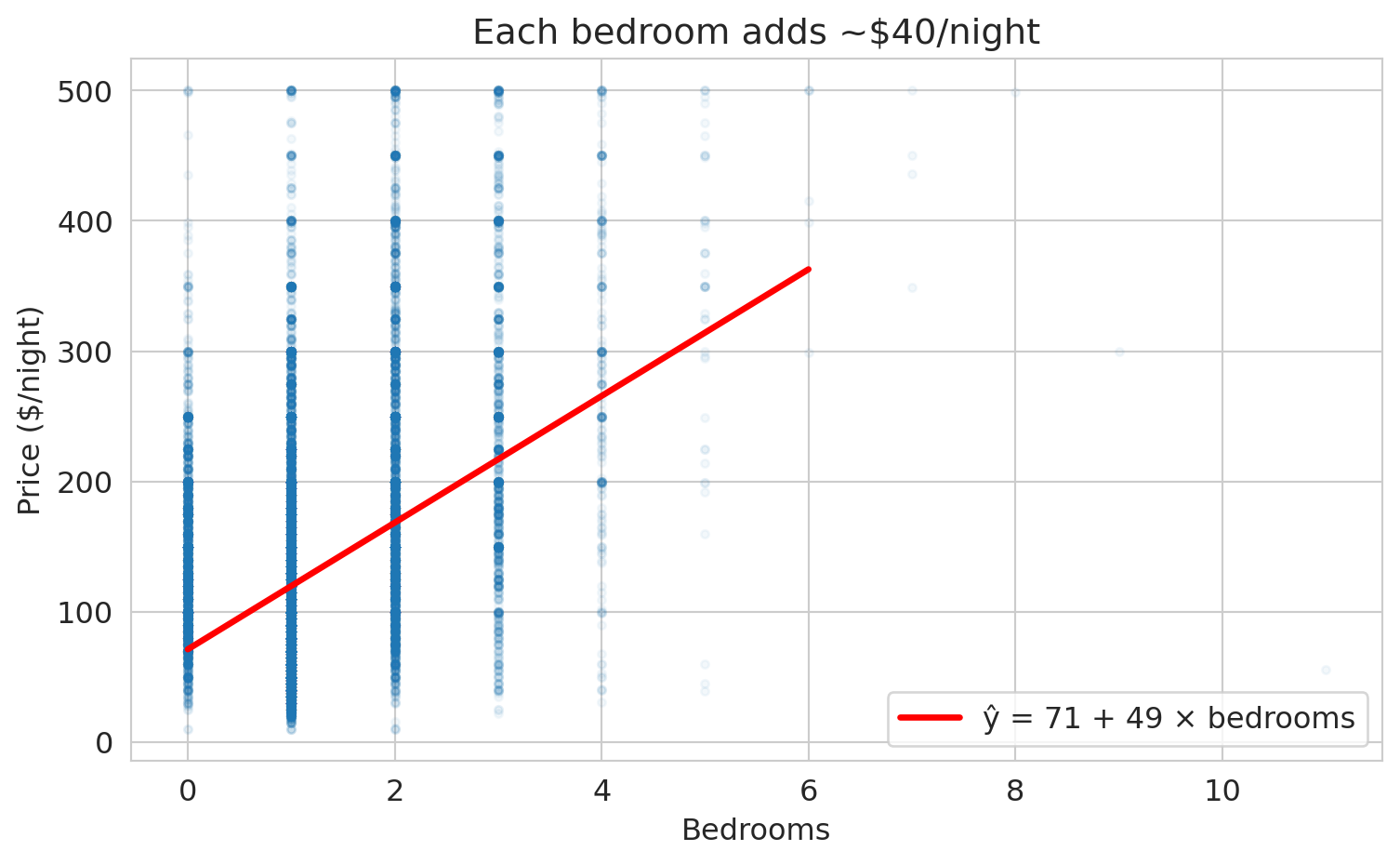
## Simple regression on Airbnb data
We already fit the simple regression $\hat{y} = \beta_0 + \beta_1 x$ above to compute the least-squares candidate line. The linear regression `model` was created with scikit-learn's `LinearRegression()`, `.fit()` found the best coefficients, and `.coef_` and `.intercept_` store the slope and intercept. Print the coefficients alongside $R^2$ and draw the fitted line on the original scatter:
```{python}
r2 = model.score(df[['bedrooms']], prices)
print(f"ŷ = {b0:.0f} + {b1:.0f} × bedrooms")
print(f"R² = {r2:.3f}")
```
```{python}
# Scatter plot with regression line
fig, ax = plt.subplots(figsize=(8, 5))
ax.scatter(df['bedrooms'], prices, alpha=0.04, s=10, color='#aaaaaa')
x_line = np.linspace(0, 6, 100)
y_line = model.predict(x_line.reshape(-1, 1))
ax.plot(x_line, y_line, color='#c44e52', lw=2.5,
        label=f'ŷ = {b0:.0f} + {b1:.0f} × bedrooms')

ax.set_xlabel('Bedrooms')
ax.set_ylabel('Price ($/night)')
ax.set_title('Simple regression: price vs. bedrooms')
ax.legend(fontsize=12, loc='upper left')
for spine in ['top', 'right']:
    ax.spines[spine].set_visible(False)
plt.tight_layout()
plt.show()
```
## Interpreting the coefficients
The intercept $\beta_0$ is the predicted price for a listing with zero bedrooms — a studio apartment. The slope $\beta_1$ is the predicted price increase per additional bedroom.
```{python}
print(f"Intercept (β₀): ${b0:.0f} — predicted price for a studio")
print(f"Slope (β₁):     ${b1:.0f} — each additional bedroom is associated")
print(f"                       with roughly ${b1:.0f} more per night")
```
To make the model tangible, plug in a few specific listings and read off the predictions directly.
```{python}
# Predict prices for a studio, one-, three-, and five-bedroom listing
for k in [0, 1, 3, 5]:
    pred = model.predict([[k]])[0]
    label = 'studio' if k == 0 else f'{k}-bedroom'
    print(f"  {label:<12} → ${pred:.0f} per night")
```
## Seeing the residuals
We can view the errors more clearly if we sort the listings by bedrooms. The bedrooms vector becomes monotonically increasing — a staircase rising from studios to 5-bedroom apartments — and $\hat{y} = \beta_0 + \beta_1 x$ becomes a rising staircase on top of the constant prediction $\bar{y}$.
```{python}
# Sort the full dataset by bedrooms so the bedrooms vector rises monotonically.
# Subsample for visual clarity (28k dots on top of each other hide the structure).
rng = np.random.default_rng(0)
sample_idx = rng.choice(len(df), size=2000, replace=False)
sample = df.iloc[sample_idx].sort_values('bedrooms').reset_index(drop=True)

idx_plot = np.arange(len(sample))
beds_sorted = sample['bedrooms'].values
price_sorted = sample['price'].values
pred_linear = b0 + b1 * beds_sorted
y_bar_sample = prices.mean()

fig, ax = plt.subplots(figsize=(9, 4.5))
ax.scatter(idx_plot, price_sorted, color='#aaaaaa', s=8, alpha=0.45,
           label='actual price $y$ (sample of 2,000)')
ax.axhline(y_bar_sample, color='#2d8a4e', lw=2, ls='--',
           label=f'constant $\\bar{{y}}$ = {y_bar_sample:.0f}')
ax.plot(idx_plot, pred_linear, color='#2d6a9f', lw=2.5,
        label=f'$\\hat{{y}} = {b0:.0f} + {b1:.0f} \\cdot$ bedrooms')

ax.set_xlabel('Listing index (sorted by bedrooms)')
ax.set_ylabel('Price ($/night)')
ax.set_title('Prediction varies with bedrooms')
ax.legend(fontsize=10, loc='upper left')
for spine in ['top', 'right']:
    ax.spines[spine].set_visible(False)
plt.tight_layout()
plt.show()
```
The flat green dashes are the constant prediction $\beta_0 \mathbf{1} = \bar{y}$ the previous section settled on. The blue staircase is the linear prediction: it matches the constant at 0 bedrooms and climbs as the bedroom count grows. The linear model absorbs the rising trend the constant could not.
:::{.callout-warning}
## Association, not causation
The regression coefficient measures a statistical association: listings with more bedrooms tend to cost more. The coefficient does not tell us that *adding* a bedroom to a fixed listing would increase its price by this amount. Larger listings differ from smaller ones in many ways — location, amenities, quality — and the bedroom coefficient may be absorbing some of those differences. We return to causal reasoning in [Chapter 18](lec18-causal-inference-1.qmd).
:::
## Verifying orthogonality
The normal equations guarantee that the residual is orthogonal to both $\mathbf{1}$ and the bedrooms column. Let's verify.
```{python}
y_hat = model.predict(df[['bedrooms']])
residuals = prices - y_hat

dot_ones = np.dot(residuals, np.ones(len(df)))
dot_beds = np.dot(residuals, df['bedrooms'].values)

print(f"residuals · 1 (ones vector):  {dot_ones:.4f}   (≈ 0)")
print(f"residuals · x (bedrooms):     {dot_beds:.4f}   (≈ 0)")
print(f"\nBoth inner products are effectively zero — orthogonality holds.")
```
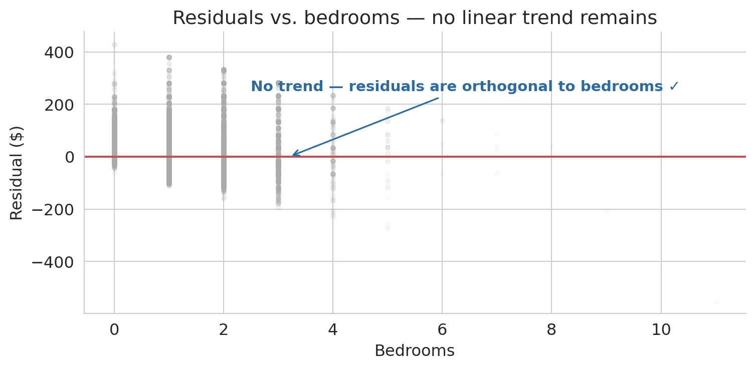
The inner products are effectively zero, so orthogonality holds algebraically. Now let us visualize what orthogonality means. If the residual is truly orthogonal to the bedrooms column, scattering residuals against bedrooms should show no remaining trend — just noise around zero.
```{python}
fig, ax = plt.subplots(figsize=(8, 4))
ax.scatter(df['bedrooms'], residuals, alpha=0.04, s=10, color='#aaaaaa')
ax.axhline(0, color='#c44e52', lw=1.5)
ax.annotate('No trend — residuals are orthogonal to bedrooms ✓',
            xy=(3.2, 0), xytext=(2.5, 250),
            fontsize=11, color='#2d6a9f', fontweight='semibold',
            arrowprops=dict(arrowstyle='->', color='#2d6a9f', lw=1.2))
ax.set_xlabel('Bedrooms')
ax.set_ylabel('Residual ($)')
ax.set_title('Residuals vs. bedrooms — no linear trend remains')
for spine in ['top', 'right']:
    ax.spines[spine].set_visible(False)
plt.tight_layout()
plt.show()
```
:::{.callout-tip}
## Think about it
The residual cloud above is flat on average, as orthogonality guarantees. But suppose the cloud curved — sagging below zero in the middle and rising at the extremes. What would a curved pattern like that tell you about the relationship between price and bedrooms? Pause and form an answer before reading on.
:::
A curved residual pattern would signal that a linear model misses systematic structure — the true relationship between price and bedrooms bends in a way that a straight line cannot follow. The remaining trend in the residuals is exactly the shape the model is failing to capture. Next lecture, we will learn techniques for expanding the model so it can absorb patterns like these.
# How good is the fit?
## $R^2$: fraction of variance explained
How much of the variation in prices does the regression explain? The prediction $\hat{y}$ splits the response into two parts: what the model captures ($\hat{y} - \bar{y}$) and what it misses (the residual $\epsilon = y - \hat{y}$).
:::{.callout-important}
## Definition: $R^2$ (coefficient of determination)
$$R^2 = 1 - \frac{\|\epsilon\|^2}{\|y - \bar{y}\|^2} = 1 - \frac{\sum_i (y_i - \hat{y}_i)^2}{\sum_i (y_i - \bar{y})^2}$$
$R^2$ measures the fraction of variance in $y$ explained by the model. A value of 0 means the model does no better than predicting $\bar{y}$ for every listing. A value of 1 means a perfect fit.
:::
```{python}
ss_res = np.sum(residuals**2)
ss_tot = np.sum((prices - prices.mean())**2)
r2 = 1 - ss_res / ss_tot

print(f"||residuals||² = {ss_res:,.0f}")
print(f"||y - ȳ||²     = {ss_tot:,.0f}")
print(f"R² = 1 - {ss_res:,.0f} / {ss_tot:,.0f} = {r2:.3f}")
print(f"\nBedrooms alone explains roughly {r2*100:.0f}% of the price variation.")
```
## $R^2$ and the angle between $y$ and $\hat{y}$
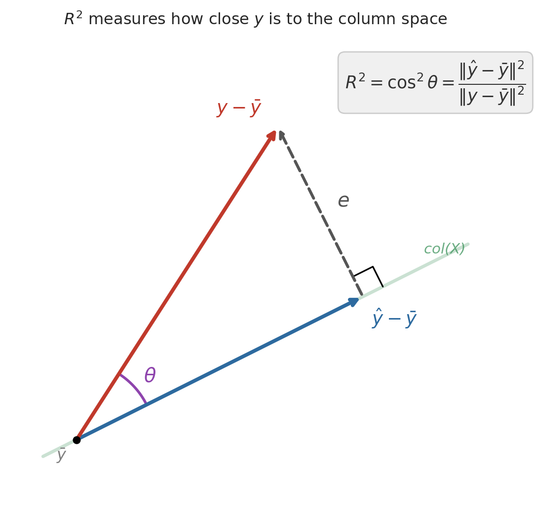
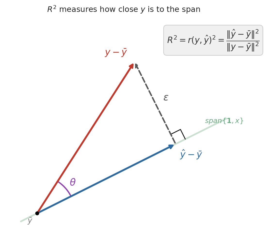
After centering $y$ (subtracting $\bar{y}$), the Pythagorean theorem gives an exact decomposition:
$$\|y - \bar{y}\|^2 = \|\hat{y} - \bar{y}\|^2 + \|\epsilon\|^2$$
The centered prediction and the residual form the two legs of a right triangle, with the centered response as the hypotenuse. Dividing through:
$$1 = \frac{\|\hat{y} - \bar{y}\|^2}{\|y - \bar{y}\|^2} + \frac{\|\epsilon\|^2}{\|y - \bar{y}\|^2} = R^2 + (1 - R^2)$$
The first ratio has a familiar name. By the definition of correlation, $\|\hat{y} - \bar{y}\| / \|y - \bar{y}\|$ is exactly $r(y, \hat{y})$ — the correlation between the actual and predicted prices. So $R^2 = r(y, \hat{y})^2$: it measures how closely the centered prediction vector aligns with the centered response, with perfect alignment ($r = \pm 1$) giving $R^2 = 1$ and orthogonal vectors ($r = 0$) giving $R^2 = 0$.
```{python}
#| code-fold: true
# R² as a projection ratio: the Pythagorean picture.
# We draw the centered response y - ȳ as one arrow, the centered
# prediction ŷ - ȳ as another, and the residual ε as the third side
# of a right triangle.
fig, ax = plt.subplots(figsize=(6, 6))

# Set up the geometry: pick a 1D span direction, and a point y off it
origin = np.array([0.0, 0.0])
col_dir = np.array([2.0, 1.0])              # direction of the feature span
y_vec = np.array([1.8, 2.8])                # centered response y - ȳ
# Project y onto the span: ŷ = (y · d / d · d) · d
yhat_vec = col_dir * (np.dot(y_vec, col_dir) / np.dot(col_dir, col_dir))
e_vec = y_vec - yhat_vec                    # residual ε (orthogonal leg)

# Draw the span as a faint line through the origin
slope = col_dir[1] / col_dir[0]
t = np.linspace(-0.3, 3.5, 100)
ax.plot(t, slope * t, color='#2d8a4e', lw=2.5, alpha=0.25)
ax.text(3.1, slope * 3.1 + 0.12, 'span$\\{\\mathbf{1}, x\\}$', fontsize=11,
        color='#2d8a4e', alpha=0.7, style='italic')

ax.annotate('', xy=yhat_vec, xytext=origin,
            arrowprops=dict(arrowstyle='->', color='#2d6a9f', lw=2.8))
ax.text(yhat_vec[0] + 0.08, yhat_vec[1] - 0.25,
        '$\\hat{y} - \\bar{y}$', fontsize=14, color='#2d6a9f', fontweight='bold')

# Hypotenuse: centered response y - ȳ
ax.annotate('', xy=y_vec, xytext=origin,
            arrowprops=dict(arrowstyle='->', color='#c0392b', lw=2.8))
ax.text(y_vec[0] - 0.55, y_vec[1] + 0.12, '$y - \\bar{y}$',
        fontsize=14, color='#c0392b', fontweight='bold')

# Other leg: residual ε connects ŷ to y
ax.annotate('', xy=y_vec, xytext=yhat_vec,
            arrowprops=dict(arrowstyle='->', color='#555555', lw=2.2, ls='--'))
mid_e = (y_vec + yhat_vec) / 2
ax.text(mid_e[0] + 0.15, mid_e[1] + 0.05, '$\\epsilon$',
        fontsize=15, color='#555555', style='italic')

# Right-angle marker at ŷ (where ε meets the span)
sz = 0.2
p_dir = col_dir / np.linalg.norm(col_dir)
r_dir = e_vec / np.linalg.norm(e_vec)
sq = np.array([yhat_vec + sz * p_dir,
               yhat_vec + sz * p_dir + sz * r_dir,
               yhat_vec + sz * r_dir])
ax.plot(sq[:, 0], sq[:, 1], 'k-', lw=1.2)

# Arc marking the angle θ between y - ȳ and ŷ - ȳ
angle_y = np.arctan2(y_vec[1], y_vec[0])
angle_yhat = np.arctan2(yhat_vec[1], yhat_vec[0])
arc_r = 0.7
theta_range = np.linspace(angle_yhat, angle_y, 40)
ax.plot(arc_r * np.cos(theta_range), arc_r * np.sin(theta_range),
        color='#8e44ad', lw=2)
mid_angle = (angle_y + angle_yhat) / 2
ax.text(arc_r * np.cos(mid_angle) + 0.08,
        arc_r * np.sin(mid_angle) + 0.05,
        '$\\theta$', fontsize=15, color='#8e44ad')

ax.text(2.4, 3.15,
        '$R^2 = r(y, \\hat{y})^2'
        ' = \\dfrac{\\|\\hat{y} - \\bar{y}\\|^2}{\\|y - \\bar{y}\\|^2}$',
        fontsize=13, color='#333333',
        bbox=dict(boxstyle='round,pad=0.4', facecolor='#f0f0f0',
                  edgecolor='#cccccc'))

ax.plot(0, 0, 'ko', ms=5, zorder=5)
ax.text(-0.18, -0.18, '$\\bar{y}$', fontsize=12, color='gray')

ax.set_xlim(-0.6, 3.8)
ax.set_ylim(-0.5, 3.6)
ax.set_aspect('equal')
for spine in ax.spines.values():
    spine.set_visible(False)
ax.set_xticks([])
ax.set_yticks([])
ax.set_title('$R^2$ measures how close $y$ is to the span',
             fontsize=12, pad=10)
plt.tight_layout()
plt.show()
```
## $R^2 = r^2$ in simple regression
For a model with **one** predictor, $R^2$ equals the square of the Pearson correlation coefficient $r$. The simple regression prediction can be written as $\hat{y}_i = \bar{y} + r \cdot \frac{SD_y}{SD_x}(x_i - \bar{x})$, so the explained variance is exactly $r^2$ times the total variance.
```{python}
r = df['price'].corr(df['bedrooms'])
print(f"Pearson correlation r = {r:.4f}")
print(f"r² = {r**2:.4f}")
print(f"R² from regression  = {r2:.4f}")
print(f"\nIn simple regression, R² = r². With multiple predictors, only R² applies.")
```
# Regression to the mean
## Galton's heights
The name "regression" has a surprising origin. In the 1880s, Francis Galton studied the heights of parents and their adult children. He noticed a striking pattern: unusually tall parents tended to have children who were tall — but *less* tall than their parents. Unusually short parents had children who were short — but *less* short. Heights "regressed toward the mean."
We can reproduce Galton's original analysis on his own data. The dataset below is Galton's 1886 family-heights dataset, recording the heights of 934 adult children from 205 families. Galton put everyone on a common scale by multiplying female heights by 1.08 (the typical male/female ratio of his era), then plotted each child's height against the **midparent height** — the average of the father's height and 1.08 times the mother's height.
```{python}
# Galton's 1886 family heights
galton = pd.read_csv(f'{DATA_DIR}/galton/galton.csv')

# Galton adjusted female heights by 1.08 to put everyone on a male scale
galton['adjusted_child'] = np.where(
    galton['gender'] == 'female',
    galton['childHeight'] * 1.08,
    galton['childHeight'])

print(f"{len(galton)} children from {galton['family'].nunique()} families")
print(f"Midparent height: mean = {galton['midparentHeight'].mean():.1f}\", "
      f"SD = {galton['midparentHeight'].std():.1f}\"")
print(f"Adjusted child height: mean = {galton['adjusted_child'].mean():.1f}\", "
      f"SD = {galton['adjusted_child'].std():.1f}\"")
```
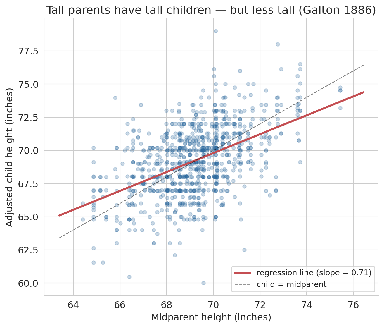
Now fit a regression of adjusted child height on midparent height and plot it against the 45-degree line ("child has the same height as the midparent").
```{python}
x_mp = galton['midparentHeight'].values
y_ch = galton['adjusted_child'].values

model_galton = LinearRegression()
model_galton.fit(x_mp.reshape(-1, 1), y_ch)
slope_g = model_galton.coef_[0]
intercept_g = model_galton.intercept_
r_g = np.corrcoef(x_mp, y_ch)[0, 1]

fig, ax = plt.subplots(figsize=(7, 6))
ax.scatter(x_mp, y_ch, alpha=0.25, s=20, color='#2d6a9f')

x_line = np.linspace(x_mp.min() - 1, x_mp.max() + 1, 100)
ax.plot(x_line, model_galton.predict(x_line.reshape(-1, 1)),
        color='#c44e52', lw=2.5,
        label=f'regression line (slope = {slope_g:.2f})')
ax.plot(x_line, x_line, 'k--', lw=1, alpha=0.5, label='child = midparent')

ax.set_xlabel("Midparent height (inches)")
ax.set_ylabel("Adjusted child height (inches)")
ax.set_title("Tall parents have tall children — but less tall (Galton 1886)")
ax.legend(fontsize=10, loc='lower right')
for spine in ['top', 'right']:
    ax.spines[spine].set_visible(False)
plt.tight_layout()
plt.show()

print(f"Correlation r = {r_g:.3f}")
print(f"Regression slope = {slope_g:.3f}  (Galton's own estimate: about 2/3)")
print(f"Intercept = {intercept_g:.2f}")
```
The regression line is flatter than the 45-degree line. Parents 2 standard deviations above average have children predicted to be only about $r \times 2$ standard deviations above average — pulled back toward the mean. Galton's own estimate of the slope was about 2/3; the slope fitted to his data is close to that value.
:::{.callout-important}
## Definition: Regression to the mean
**Regression to the mean** is the phenomenon whereby extreme observations tend to be followed by less extreme ones. The effect arises whenever the correlation between two measurements is imperfect ($|r| < 1$). The predicted value $\hat{y}$ is always closer to $\bar{y}$ (in standardized units) than $x$ is to $\bar{x}$. This phenomenon is purely statistical — not biological or causal.
:::
Galton's method for quantifying the trend — fitting a line through the data — became known as "regression," and the name stuck even though we now use it for problems that have nothing to do with reverting to averages. (For the full story, see Salsburg, *The Lady Tasting Tea*, Ch. 4.)
:::{.callout-tip}
## Think about it
Where else do you see regression to the mean? Consider: a sports team wins 90% of games one season. Would you expect the same record next year? A student scores in the 99th percentile on one exam — will they do the same on the next?
:::
The mechanism in both cases is the same. A 90% win rate is part skill and part luck: the team is probably very good, but they also caught some breaks. Next season the skill carries over but the luck resets, so the record drifts back toward the team's underlying ability — not because the team got worse, but because an unusual streak has no reason to persist. The same logic explains the exam. Scoring in the 99th percentile reflects real knowledge plus a run of favorable questions and good guesses; the knowledge holds on the next test, but the favorable run does not. Whenever the correlation between two measurements is less than 1, extreme observations on one will, on average, look less extreme on the other.
# Closing
## From the mean to simple regression
This chapter built predictions in two stages:
1. **No features (1 parameter).** The best constant prediction is the mean $\bar{y}$. The residual is orthogonal to the ones vector: $\mathbf{1}^T \epsilon = 0$.
2. **One feature (2 parameters).** The best linear prediction $\hat{y} = \beta_0 + \beta_1 x$ is the orthogonal projection of $y$ onto span$\{\mathbf{1}, x\}$. The residual satisfies $\mathbf{1}^T \epsilon = 0$ *and* $x^T \epsilon = 0$.
The principle is the same in both cases: minimize squared error, which amounts to making the residual orthogonal to every feature. $R^2$ measures how much of $y$ lives in the feature span — geometrically, $\cos^2\theta$ of the angle between $y$ and $\hat{y}$.
In [Chapter 5](lec05-feature-engineering.qmd), we add more features — bathrooms, room type, neighborhood — and discover that the same orthogonality principle scales to any number of predictors. More features expand the span, giving the projection a chance to get closer to $y$. We will also transform raw data into features a linear model can use: one-hot encoding for categories, polynomials for nonlinear patterns, and log transforms for multiplicative relationships.
## Study guide
### Key ideas
- **Vector** — an ordered list of numbers. Each feature column is a vector in $\mathbb{R}^n$; each data row is a vector in $\mathbb{R}^d$.
- **Norm** — $\|v\| = \sqrt{\sum v_i^2}$, the length of a vector. Norms measure magnitude.
- **Distance** — $d(u,v) = \|u - v\|$, the norm of the difference vector.
- **Inner product** — $u^T v = \sum u_i v_i$. Positive means same direction; zero means orthogonal.
- **Correlation** — Pearson's $r(u, v)$ is the inner product of the centered, length-normalized vectors, ranging from $-1$ (opposite) to $+1$ (aligned). Unitless: rescaling a column leaves $r$ unchanged.
- **Linear combination** — $\beta_1 v_1 + \beta_2 v_2$, a weighted sum of vectors.
- **Span** — the set of all linear combinations of a set of vectors. Determines what a linear model can predict.
- **Orthogonal** — vectors with zero inner product. Orthogonality of the residual to the features is the optimality condition for least squares.
- **Projection** — the closest point in a subspace to $y$. Regression finds the projection of $y$ onto the span of the feature columns.
- **Residual** — $\epsilon = y - \hat{y}$, the part of $y$ the model cannot explain. Orthogonal to every feature column.
- **Normal equations** — $\mathbf{1}^T \epsilon = 0$ and $x^T \epsilon = 0$ for simple regression. The algebraic expression of the orthogonality conditions.
- **$R^2$** — fraction of variance explained; $R^2 = 1 - \|\epsilon\|^2 / \|y - \bar{y}\|^2$. Equivalently, $R^2 = r(y, \hat{y})^2$.
- **$R^2 = r^2$ in simple regression** — the correlation coefficient $r$ measures linear association ($-1$ to $+1$); $R^2$ measures variance explained ($0$ to $1$). For one predictor, squaring $r$ gives $R^2$.
- **Regression to the mean** — extreme observations tend to be followed by less extreme ones whenever $|r| < 1$.
- **Coefficient interpretation** — $\beta_0$ is the predicted $y$ when $x = 0$; $\beta_1$ is the predicted change in $y$ per unit change in $x$. Association, not causation.
### Computational tools
- `np.dot(u, v)` or `u @ v` — inner product (dot product)
- `np.linalg.norm(v)` — Euclidean norm (length) of a vector
- `LinearRegression()` — create a linear regression model (scikit-learn)
- `.fit(X, y)` — fit the model to data
- `.predict(X)` — generate predictions
- `.coef_` — fitted slope(s)
- `.intercept_` — fitted intercept
- `.score(X, y)` — compute $R^2$
- `df['col1'].corr(df['col2'])` — Pearson correlation coefficient
### For the quiz
- Given a scatter plot, sketch the regression line and identify $\beta_0$ and $\beta_1$.
- Interpret a regression coefficient in context ("each additional bedroom is associated with...").
- Explain why the mean minimizes squared error (one-line calculus argument).
- State the orthogonality conditions for simple regression and explain what each condition means.
- Compute $R^2$ from sums of squares and interpret the result.
- Identify regression to the mean in a described scenario.