---
title: "Appendix: Probability Refresher"
execute:
enabled: true
jupyter: python3
---
```{python}
import numpy as np
import pandas as pd
import matplotlib.pyplot as plt
import seaborn as sns
from scipy.stats import norm, binom, expon, multivariate_normal
sns.set_style('whitegrid')
plt.rcParams['figure.figsize'] = (7, 4.5)
plt.rcParams['font.size'] = 12
np.random.seed(42)
```
Every model in this book rests on a handful of probability ideas. This appendix is a refresher — not a replacement — for a probability course (e.g., MS&E 120 or equivalent). If any of these ideas feel rusty, work through the corresponding section below. It should take about 30--45 minutes to read in full, or about 15 minutes if you're skimming sections where you feel confident.
We don't cover moment generating functions, joint density calculations, or measure-theoretic foundations here — they won't appear in this course.
:::{.callout-important}
## Notation convention
Throughout this book, $\text{Normal}(\mu, \sigma)$ denotes a normal distribution with mean $\mu$ and **standard deviation** $\sigma$ — not variance. So $\text{Normal}(100, 15)$ means mean 100 and standard deviation 15.
:::
## Self-assessment quiz
Answer these 12 questions before reading further. If you get 10 or more right, you're ready — but if you missed any of Q7--Q11, read those sections even if your total score is high, since those concepts are critical for Act 2.
:::{.callout-tip}
## Quiz
1. You roll a fair die. What is $E[X]$, the expected value of the outcome?
2. A random variable $X$ takes values 0 and 1 with equal probability. What is $\text{Var}(X)$?
3. If $X \sim \text{Normal}(100, 15)$ (mean 100, standard deviation 15), roughly what fraction of values fall between 70 and 130?
4. You flip a fair coin 10 times. What distribution does the number of heads follow, and what is its expected value?
5. If $P(A) = 0.3$ and $P(B \mid A) = 0.8$, what is $P(A \text{ and } B)$?
6. Events $A$ and $B$ are independent. $P(A) = 0.4$, $P(B) = 0.5$. What is $P(A \text{ and } B)$?
7. You draw 100 observations iid from a distribution with mean $\mu$ and standard deviation $\sigma = 10$. What is the standard deviation of the sample mean $\bar{X}$?
8. The Law of Large Numbers says that as $n \to \infty$, the sample mean converges to _______.
9. The Central Limit Theorem says that the distribution of the sample mean approaches _______ as $n$ grows, regardless of the population shape.
10. If $\text{Cov}(X, Y) > 0$, what does that tell you about the relationship between $X$ and $Y$?
11. Let $X$ be the number showing on a fair die and let $Y$ be the number showing on a second independent fair die. What is $E[3X + Y]$?
12. If 1% of emails are spam and a filter catches 90% of spam but flags 5% of legitimate email, what fraction of flagged emails are actually spam?
:::
:::{.callout-note collapse="true"}
## Answers
1. $E[X] = (1 + 2 + 3 + 4 + 5 + 6)/6 = 3.5$
2. $\text{Var}(X) = E[X^2] - (E[X])^2 = 0.5 - 0.25 = 0.25$
3. About 95% (within two standard deviations of the mean)
4. $\text{Binomial}(10, 0.5)$ with expected value $np = 5$
5. $P(A \text{ and } B) = P(A) \cdot P(B \mid A) = 0.3 \times 0.8 = 0.24$
6. $P(A \text{ and } B) = P(A) \cdot P(B) = 0.4 \times 0.5 = 0.2$ (independence means we can multiply)
7. $\sigma / \sqrt{n} = 10 / \sqrt{100} = 1$
8. The population mean $\mu$
9. A normal distribution (specifically $\text{Normal}(\mu, \sigma/\sqrt{n})$)
10. $X$ and $Y$ tend to move in the same direction — when $X$ is above its mean, $Y$ tends to be above its mean too
11. By linearity of expectation, $E[3X + Y] = 3E[X] + E[Y] = 3(3.5) + 3.5 = 14$
12. About 15%. By Bayes' rule: $P(\text{spam} \mid \text{flagged}) = \frac{0.90 \times 0.01}{0.90 \times 0.01 + 0.05 \times 0.99} \approx 0.154$. Most flagged emails are false alarms because spam is rare.
:::
## Concepts you'll need
The rest of this appendix covers twelve ideas, grouped into four clusters:
| Cluster | Concepts | Where they appear |
|---------|----------|-------------------|
| **Random variables** | random variables, probability distributions | throughout |
| **Summaries** | expected value, variance, covariance | throughout, especially Chapters 5--14 |
| **Named distributions** | normal, binomial, uniform | Chapters 8--13 |
| **Convergence & sampling** | independence, iid, LLN, CLT, sampling distributions | Chapters 8--12 |
## Random variables
You measure the height of a randomly chosen Stanford student — call that $X$. Before you measure, $X$ is uncertain: it's a **random variable**. We write it with a capital letter to distinguish it from a fixed number $x$.
- **Discrete** random variables take on a countable set of values: the number of heads in 10 coin flips, the number of patients in a clinical trial who respond to treatment.
- **Continuous** random variables can take any value in an interval: a patient's blood pressure, the price of a rental listing.
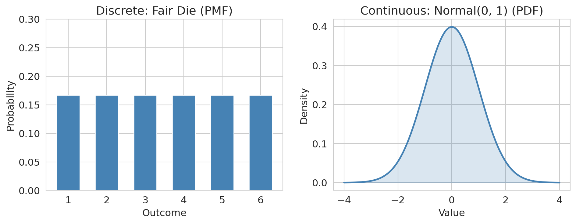
The distinction matters for how we assign probabilities: discrete random variables have **probability mass functions** (PMFs) while continuous ones have **probability density functions** (PDFs). The intuition is the same — both tell you which values are more or less likely.
### Probability distributions
A **probability distribution** assigns probabilities to the possible values of a random variable. For a discrete variable:
$$P(X = x) = p(x) \quad \text{(the PMF)}$$
For a continuous variable, the probability of landing in an interval is the area under the curve:
$$P(a \le X \le b) = \int_a^b f(x) \, dx \quad \text{(where } f \text{ is the PDF)}$$
The **cumulative distribution function** (CDF) works for both:
$$F(x) = P(X \le x)$$
```{python}
fig, axes = plt.subplots(1, 2, figsize=(10, 4))

# Discrete: rolling a die
outcomes = np.arange(1, 7)
probs = np.ones(6) / 6
axes[0].bar(outcomes, probs, color='steelblue', edgecolor='white', width=0.6)
axes[0].set_xlabel('Outcome')
axes[0].set_ylabel('Probability')
axes[0].set_title('Discrete: Fair Die (PMF)')
axes[0].set_ylim(0, 0.3)
axes[0].set_xticks(outcomes)

# Continuous: normal distribution
x = np.linspace(-4, 4, 200)
axes[1].plot(x, norm.pdf(x), color='steelblue', lw=2)
axes[1].fill_between(x, norm.pdf(x), alpha=0.2, color='steelblue')
axes[1].set_xlabel('Value')
axes[1].set_ylabel('Density')
axes[1].set_title('Continuous: Normal(0, 1) (PDF)')

plt.tight_layout()
plt.show()
```
Notice the y-axis label: **probability** for the discrete case, **density** for the continuous case. A PDF value can exceed 1 — it's not a probability. Only the *area* under the curve over an interval gives a probability.
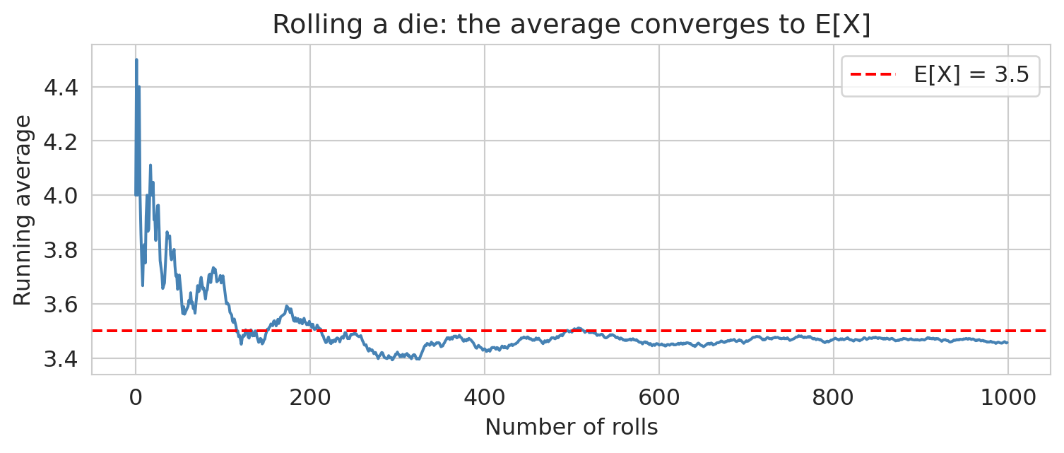
## Expected value
The **expected value** (or **mean**) of a random variable is its long-run average:
$$E[X] = \sum_x x \cdot P(X = x) \quad \text{(discrete)} \qquad E[X] = \int_{-\infty}^{\infty} x \cdot f(x) \, dx \quad \text{(continuous)}$$
It's a weighted average of the possible values, weighted by their probabilities.
```{python}
# Simulate: roll a die many times, track the running average
rolls = np.random.randint(1, 7, size=1000)
running_avg = np.cumsum(rolls) / np.arange(1, 1001)

plt.figure(figsize=(8, 3.5))
plt.plot(running_avg, color='steelblue', lw=1.5)
plt.axhline(3.5, color='red', ls='--', lw=1.5, label='E[X] = 3.5')
plt.xlabel('Number of rolls')
plt.ylabel('Running average')
plt.title('Rolling a die: the average converges to E[X]')
plt.legend()
plt.tight_layout()
plt.show()
```
The running average settles down near 3.5 — that's the Law of Large Numbers in action (more on that below).
Two useful properties you'll see throughout this book:
- **Linearity of expectation:** $E[aX + bY] = aE[X] + bE[Y]$, always — even when $X$ and $Y$ are dependent. Linearity of expectation allows us to compute the expected number of false positives in Chapter 11 without knowing the dependence structure of our test statistics.
- **Conditional expectation:** $E[X \mid Y = y]$ is the expected value of $X$ given that $Y$ takes the value $y$. For example, the expected points per shot from mid-range is a conditional expectation — the mean outcome conditioned on shot location.
## Variance and standard deviation
**Variance** measures how spread out a random variable is around its mean:
$$\text{Var}(X) = E\big[(X - E[X])^2\big] = E[X^2] - (E[X])^2$$
The **standard deviation** is $\text{SD}(X) = \sqrt{\text{Var}(X)}$, which has the same units as $X$.
```{python}
x = np.linspace(-6, 10, 300)
plt.figure(figsize=(8, 3.5))
plt.plot(x, norm.pdf(x, loc=2, scale=1), lw=2, label='SD = 1 (tight)')
plt.plot(x, norm.pdf(x, loc=2, scale=3), lw=2, label='SD = 3 (spread out)')
plt.axvline(2, color='gray', ls=':', lw=1)
plt.xlabel('Value')
plt.ylabel('Density')
plt.title('Same mean, different variance')
plt.legend()
plt.tight_layout()
plt.show()
```
Key properties:
- $\text{Var}(aX + b) = a^2 \text{Var}(X)$ — shifting by $b$ doesn't change spread; scaling by $a$ scales variance by $a^2$.
- For **independent** random variables: $\text{Var}(X + Y) = \text{Var}(X) + \text{Var}(Y)$.
:::{.callout-note}
## Looking ahead
In the bias-variance decomposition (Chapter 6), the "variance" term is exactly $\text{Var}(\hat{f}(x))$ — how much the model's prediction varies across different training sets.
:::
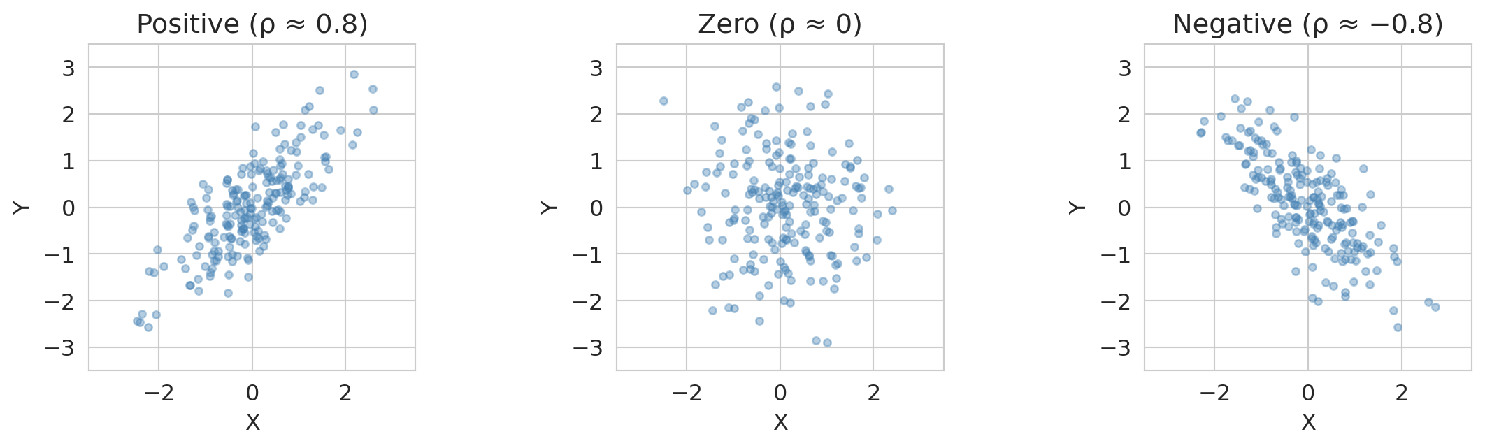
## Covariance and correlation
**Covariance** measures how two random variables move together:
$$\text{Cov}(X, Y) = E\big[(X - E[X])(Y - E[Y])\big] = E[XY] - E[X]E[Y]$$
- Positive covariance: $X$ and $Y$ tend to be above (or below) their means together.
- Negative covariance: when one is above its mean, the other tends to be below.
- Zero covariance: no *linear* relationship (but there could be a nonlinear one).
**Correlation** is covariance normalized to $[-1, 1]$:
$$\rho(X, Y) = \frac{\text{Cov}(X, Y)}{\text{SD}(X) \cdot \text{SD}(Y)}$$
:::{.callout-note}
## Looking ahead
The population correlation $\rho$ is the theoretical version of Pearson's $r$, which you'll compute from data in Chapter 11.
:::
The key advantage of correlation over covariance: it's unitless, so $\rho = 0.8$ means the same thing whether we're measuring height in centimeters or inches.
```{python}
fig, axes = plt.subplots(1, 3, figsize=(12, 3.5))
titles = ['Positive (ρ ≈ 0.8)', 'Zero (ρ ≈ 0)', 'Negative (ρ ≈ −0.8)']
covs = [[[1, 0.8], [0.8, 1]], [[1, 0], [0, 1]], [[1, -0.8], [-0.8, 1]]]

for ax, title, cov in zip(axes, titles, covs):
    data = np.random.multivariate_normal([0, 0], cov, size=200)
    ax.scatter(data[:, 0], data[:, 1], alpha=0.4, s=15, color='steelblue')
    ax.set_title(title)
    ax.set_xlabel('X')
    ax.set_ylabel('Y')
    ax.set_xlim(-3.5, 3.5)
    ax.set_ylim(-3.5, 3.5)
    ax.set_aspect('equal')

plt.tight_layout()
plt.show()
```
Important: if $X$ and $Y$ are **independent**, then $\text{Cov}(X, Y) = 0$. The converse is not true — zero covariance does not imply independence. The classic counterexample: if $X \sim \text{Normal}(0,1)$ and $Y = X^2$, then $\text{Cov}(X, Y) = 0$ even though $Y$ is completely determined by $X$.
Now we turn from summaries of random variables to the three named distributions you'll encounter most often.
## The normal distribution
The **normal** (Gaussian) distribution is the single most important distribution in this course. A normal random variable with mean $\mu$ and standard deviation $\sigma$ is written $X \sim \text{Normal}(\mu, \sigma)$.
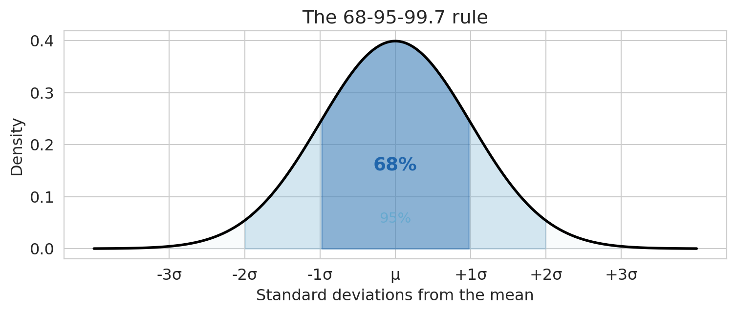
The key fact to remember is the **68-95-99.7 rule**:
- About 68% of values fall within $\pm 1\sigma$ of the mean
- About 95% fall within $\pm 2\sigma$
- About 99.7% fall within $\pm 3\sigma$
```{python}
x = np.linspace(-4, 4, 300)
y = norm.pdf(x)

fig, ax = plt.subplots(figsize=(8, 3.5))
ax.plot(x, y, 'k', lw=2)

# Shade the three regions
ax.fill_between(x, y, where=(x > -3) & (x < 3), alpha=0.15, color='#d1e5f0')
ax.fill_between(x, y, where=(x > -2) & (x < 2), alpha=0.25, color='#67a9cf')
ax.fill_between(x, y, where=(x > -1) & (x < 1), alpha=0.4, color='#2166ac')

ax.set_xlabel('Standard deviations from the mean')
ax.set_ylabel('Density')
ax.set_title('The 68-95-99.7 rule')
ax.set_xticks([-3, -2, -1, 0, 1, 2, 3])
ax.set_xticklabels(['-3σ', '-2σ', '-1σ', 'μ', '+1σ', '+2σ', '+3σ'])
ax.annotate('68%', xy=(0, 0.15), fontsize=14, ha='center', fontweight='bold', color='#2166ac')
ax.annotate('95%', xy=(0, 0.05), fontsize=11, ha='center', color='#67a9cf')

plt.tight_layout()
plt.show()
```
The **standard normal** is the special case $Z \sim \text{Normal}(0, 1)$. Any normal can be standardized: if $X \sim \text{Normal}(\mu, \sigma)$, then $Z = (X - \mu)/\sigma$ is standard normal. The number 1.96 that appears throughout Chapters 8--12 is the critical value where $P(Z > 1.96) = 0.025$ — so 95% of the standard normal falls between $-1.96$ and $+1.96$.
For reference, the PDF of the normal distribution is the bell curve formula:
$$f(x) = \frac{1}{\sigma\sqrt{2\pi}} \exp\!\left(-\frac{(x - \mu)^2}{2\sigma^2}\right)$$
You don't need to memorize this — the 68-95-99.7 rule and standardization are what you'll actually use.
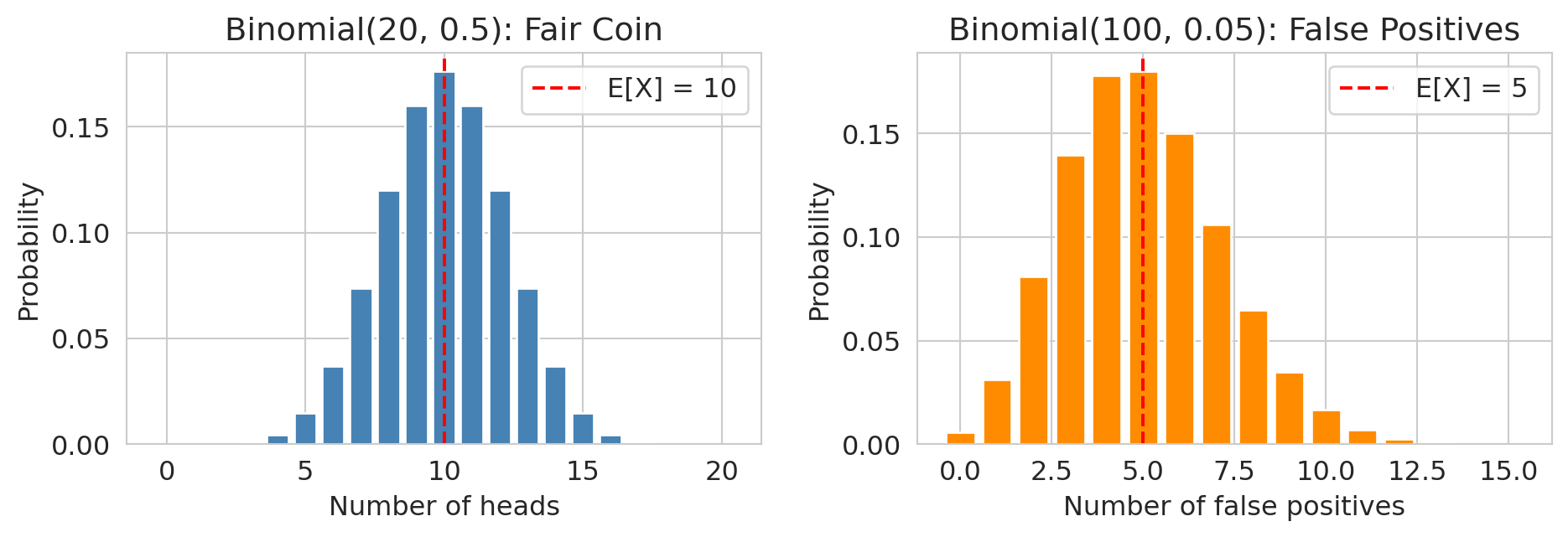
## The binomial distribution
The **binomial** distribution counts successes in independent trials. If you run $n$ independent trials, each with success probability $p$, the number of successes $X$ follows:
$$X \sim \text{Binomial}(n, p) \qquad P(X = k) = \binom{n}{k} p^k (1-p)^{n-k}$$
Key facts:
- $E[X] = np$
- $\text{Var}(X) = np(1-p)$
The special case $n = 1$ is the **Bernoulli distribution**: $X \sim \text{Bernoulli}(p)$ takes value 1 with probability $p$ and 0 with probability $1 - p$. You'll see this in Chapter 7, where each patient either has coronary heart disease or doesn't — a single Bernoulli trial.
```{python}
fig, axes = plt.subplots(1, 2, figsize=(10, 3.5))

# Coin flips
k = np.arange(0, 21)
axes[0].bar(k, binom.pmf(k, 20, 0.5), color='steelblue', edgecolor='white')
axes[0].set_xlabel('Number of heads')
axes[0].set_ylabel('Probability')
axes[0].set_title('Binomial(20, 0.5): Fair Coin')
axes[0].axvline(10, color='red', ls='--', lw=1.5, label='E[X] = 10')
axes[0].legend()

# False positives: 100 tests at alpha=0.05
k2 = np.arange(0, 16)
axes[1].bar(k2, binom.pmf(k2, 100, 0.05), color='darkorange', edgecolor='white')
axes[1].set_xlabel('Number of false positives')
axes[1].set_ylabel('Probability')
axes[1].set_title('Binomial(100, 0.05): False Positives')
axes[1].axvline(5, color='red', ls='--', lw=1.5, label='E[X] = 5')
axes[1].legend()

plt.tight_layout()
plt.show()
```
:::{.callout-note}
## Looking ahead
In Chapter 11, if you run 100 hypothesis tests and all null hypotheses are true, the number of false rejections follows $\text{Binomial}(100, 0.05)$ — you expect 5 false positives by chance alone.
:::
## The uniform distribution
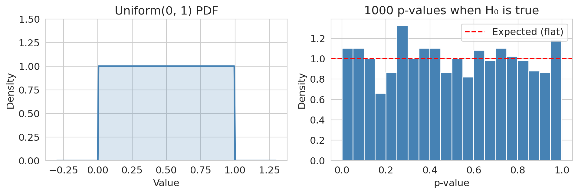
A **uniform** random variable is equally likely to take any value in an interval:
$$X \sim \text{Uniform}(a, b) \qquad f(x) = \frac{1}{b - a} \text{ for } a \le x \le b$$
With $E[X] = (a+b)/2$ and $\text{Var}(X) = (b-a)^2/12$.
:::{.callout-note}
## Looking ahead
A key fact for Act 2: **p-values are Uniform(0, 1) when the null hypothesis is true.** A uniform p-value histogram means no signal; a spike near zero means some effects are real. You'll use this diagnostic in Chapters 9--11.
:::
```{python}
fig, axes = plt.subplots(1, 2, figsize=(10, 3.5))

# Uniform PDF
x = np.linspace(-0.3, 1.3, 300)
axes[0].plot(x, np.where((x >= 0) & (x <= 1), 1, 0), color='steelblue', lw=2)
axes[0].fill_between(x, np.where((x >= 0) & (x <= 1), 1, 0), alpha=0.2, color='steelblue')
axes[0].set_xlabel('Value')
axes[0].set_ylabel('Density')
axes[0].set_title('Uniform(0, 1) PDF')
axes[0].set_ylim(0, 1.5)

# P-values under null
p_values = np.random.uniform(0, 1, size=1000)
axes[1].hist(p_values, bins=20, color='steelblue', edgecolor='white', density=True)
axes[1].axhline(1, color='red', ls='--', lw=1.5, label='Expected (flat)')
axes[1].set_xlabel('p-value')
axes[1].set_ylabel('Density')
axes[1].set_title('1000 p-values when H₀ is true')
axes[1].legend()

plt.tight_layout()
plt.show()
```
The final cluster of concepts is about what happens when you collect many observations and try to draw conclusions from them.
## Independence
Two random variables $X$ and $Y$ are **independent** if knowing the value of one tells you nothing about the other:
$$P(X = x \text{ and } Y = y) = P(X = x) \cdot P(Y = y) \quad \text{for all } x, y$$
Equivalently, $P(Y = y \mid X = x) = P(Y = y)$ — conditioning on $X$ doesn't change the distribution of $Y$. In plain language, $X$ *doesn't affect* $Y$ (and vice versa). (For continuous random variables, the same idea holds with densities in place of probabilities.)
Independence simplifies everything:
- $E[XY] = E[X] \cdot E[Y]$
- $\text{Var}(X + Y) = \text{Var}(X) + \text{Var}(Y)$
- $\text{Cov}(X, Y) = 0$
:::{.callout-warning}
## Independence is an assumption, not a fact
In practice, independence is an assumption. We sometimes try to check independence, but it can be difficult to infer from data! In Chapter 8, the bootstrap assumes observations are independent. In Chapter 19, A/B tests require that one user's outcome doesn't affect another's (the "no interference" condition). When independence fails — social networks, spatial data, time series — standard tools can give misleading answers.
:::
## iid: independent and identically distributed
The most common assumption in statistics combines two ideas:
- **Independent:** each observation is drawn without being influenced by any other.
- **Identically distributed:** each observation is drawn from the same probability distribution.
Together, **iid** means: every data point in your sample was generated by the same random process, and they don't affect each other. The iid assumption underlies the bootstrap (Chapter 8) and most of the inference tools in Act 2.
When does iid fail?
- **Time series data:** today's air quality depends on yesterday's — observations are not independent.
- **Clustered data:** students in the same school share a common environment — they're not independent.
- **Distribution shift:** if the data-generating process changes over time, observations are not identically distributed.
## The Law of Large Numbers
The **Law of Large Numbers** (LLN) says that the sample mean converges (in probability) to the population mean as the sample size grows:
$$\bar{X}_n = \frac{1}{n}\sum_{i=1}^n X_i \xrightarrow{n \to \infty} E[X]$$
provided the $X_i$ are iid with finite mean.
The LLN provides the formal justification for something intuitive: flip a coin enough times and the fraction of heads approaches 0.5. It's also why bigger samples give more reliable estimates — the running average plot in the Expected Value section illustrates LLN in action.
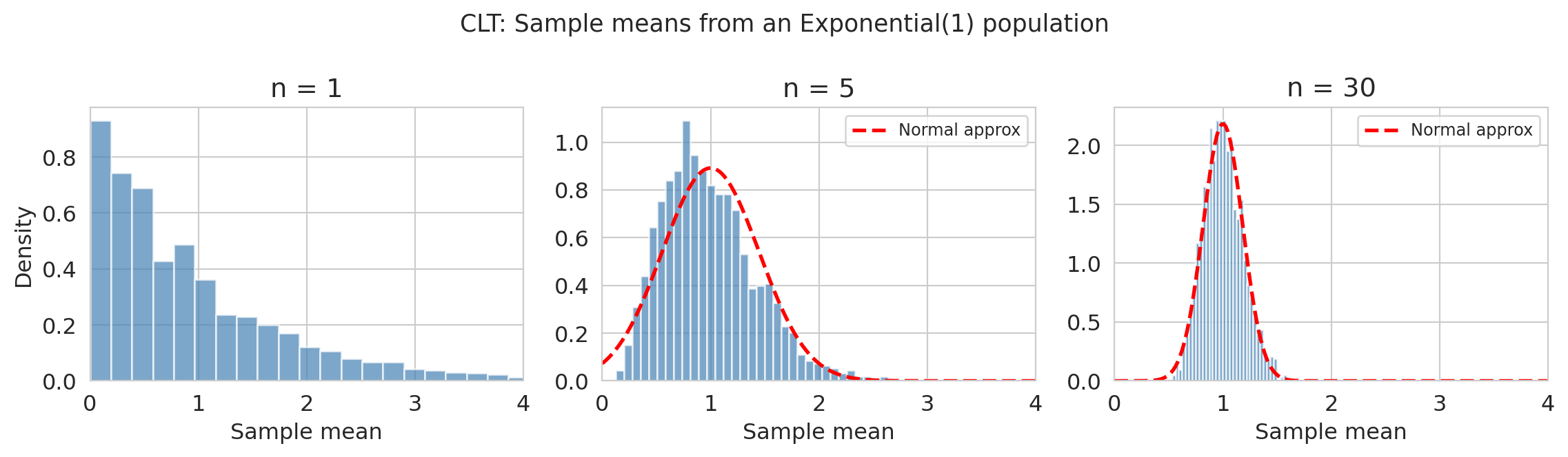
## The Central Limit Theorem
The **Central Limit Theorem** (CLT) is perhaps the most important result in probability for applied statistics. It says that the *distribution* of the sample mean approaches a normal distribution, regardless of the population shape:
$$\bar{X}_n \approx \text{Normal}\!\left(\mu, \frac{\sigma}{\sqrt{n}}\right) \quad \text{for large } n$$
provided the $X_i$ are iid with finite mean $\mu$ and finite variance $\sigma^2$.
The quantity $\sigma / \sqrt{n}$ is the **standard error** — it tells you how precisely the sample mean estimates the population mean. Double the sample size, and the standard error shrinks by a factor of $\sqrt{2}$.
```{python}
fig, axes = plt.subplots(1, 3, figsize=(12, 3.5))
sample_sizes = [1, 5, 30]

for ax, n in zip(axes, sample_sizes):
    # Vectorized: draw 2000 samples of size n from Exponential(1)
    means = np.random.exponential(1, size=(2000, n)).mean(axis=1)
    ax.hist(means, bins=40, density=True, color='steelblue', edgecolor='white', alpha=0.7)
    ax.set_title(f'n = {n}')
    ax.set_xlabel('Sample mean')
    ax.set_xlim(0, 4)
    if n >= 5:
        xfit = np.linspace(0, 4, 200)
        ax.plot(xfit, norm.pdf(xfit, loc=1, scale=1/np.sqrt(n)),
                'r--', lw=2, label='Normal approx')
        ax.legend(fontsize=9)

axes[0].set_ylabel('Density')
plt.suptitle('CLT: Sample means from an Exponential(1) population', fontsize=13)
plt.tight_layout()
plt.show()
```
The population here is Exponential(1) — visibly skewed. But by $n = 30$, the distribution of sample means is nearly bell-shaped. The CLT explains why the normal distribution shows up everywhere in Chapters 8--12, even when the underlying data aren't normal: we're usually looking at *averages* (or functions of averages), and the CLT guarantees those are approximately normal.
:::{.callout-important}
## What the CLT requires
The CLT needs:
- **iid** observations (or at least weak dependence and identical distributions)
- **Finite variance** — if the population variance is infinite (as with Cauchy or other stable distributions), the CLT doesn't apply
- **Large enough $n$** — "large enough" depends on how skewed the population is. For symmetric populations, $n = 10$ often suffices. For highly skewed ones, you may need $n = 100$ or more.
:::
## Sampling distributions and standard errors
The CLT is a specific instance of a broader idea: any statistic you compute from random data — a mean, a median, a regression coefficient — is itself a random variable. Compute it on a different sample, and you'll get a different number.
The **sampling distribution** of a statistic is the distribution of values that statistic would take across all possible samples from the population. You can't observe it directly (you only have one sample), but the bootstrap (Chapter 8) approximates it by resampling.
The **standard error** of a statistic is the standard deviation of its sampling distribution — it measures how much the statistic varies from sample to sample. For a sample mean, the CLT gives us a formula: $\text{SE}(\bar{X}) = \sigma / \sqrt{n}$. For other statistics (medians, regression coefficients, etc.), we typically estimate the standard error via the bootstrap.
These two concepts — sampling distributions and standard errors — are the foundation of all the inference tools in Act 2 (Chapters 8--12). Whenever you see a confidence interval or a p-value, there's a sampling distribution and a standard error behind it.
You'll also encounter the **$t$-distribution** starting in Chapter 10: it looks like a normal distribution but with heavier tails, and it arises when you replace the unknown population standard deviation $\sigma$ with the sample standard deviation $s$ — which is almost always necessary in practice. As the sample size grows, the $t$-distribution converges to the normal — another instance of the CLT at work.
## Conditional probability
The **conditional probability** of $A$ given $B$ is:
$$P(A \mid B) = \frac{P(A \text{ and } B)}{P(B)}$$
It answers the question: if I know $B$ happened, how does that update my belief about $A$? Here $A$ and $B$ can be any events, including events defined in terms of random variables like $\{X > 5\}$ or $\{Y = 1\}$.
Two derived rules you'll use implicitly throughout the book:
- **Multiplication rule:** $P(A \text{ and } B) = P(A) \cdot P(B \mid A)$
- **Bayes' rule:** $P(A \mid B) = \frac{P(B \mid A) \cdot P(A)}{P(B)}$
:::{.callout-note}
## Looking ahead
Conditional probability is the engine behind classification (Chapter 7), where logistic regression estimates $P(\text{disease} \mid \text{features})$, and causal inference (Chapters 18--19), where conditioning on confounders changes the conditional distribution of the outcome. The closely related **likelihood function**, $P(\text{data} \mid \theta)$, reverses the conditioning — you'll see this formulation in Chapters 5 and 7.
:::
```{python}
# Spam filter example: Bayes' rule in action
prevalence = 0.01       # 1% of emails are spam
sensitivity = 0.90      # filter catches 90% of spam
false_alarm = 0.05      # filter flags 5% of legitimate email

# P(flagged) = P(flagged | spam) * P(spam) + P(flagged | legit) * P(legit)
p_flagged = sensitivity * prevalence + false_alarm * (1 - prevalence)

# Bayes' rule: P(spam | flagged)
p_spam_given_flagged = (sensitivity * prevalence) / p_flagged

print("Spam filter with Bayes' rule")
print(f"  Spam prevalence:       {prevalence:.0%}")
print(f"  Filter sensitivity:    {sensitivity:.0%}")
print(f"  False alarm rate:      {false_alarm:.0%}")
print(f"  P(email flagged):      {p_flagged:.1%}")
print(f"  P(spam | flagged):     {p_spam_given_flagged:.1%}")
print(f"\nEven with a good filter, only {p_spam_given_flagged:.0%} of flagged emails")
print("are actually spam — because spam is rare (the 'base rate').")
```
This "base rate" effect — where a low prior probability dominates even a good classifier — shows up whenever you interpret predictions on imbalanced data (Chapter 7). A model with 95% accuracy can still be mostly wrong on the rare class.
## Summary
| Concept | Notation | Where it matters most |
|---------|----------|----------------------|
| Random variable | $X$ | throughout |
| Expected value | $E[X]$ | throughout, especially Chapters 5--8, 11 |
| Variance | $\text{Var}(X)$ | Chapters 5, 7--8, 12, 14 |
| Covariance | $\text{Cov}(X, Y)$ | Chapters 2, 5, 11, 14 |
| Normal distribution | $\text{Normal}(\mu, \sigma)$ | Chapters 8--13 |
| Binomial / Bernoulli | $\text{Bin}(n, p)$ | Chapters 11, 13 |
| Uniform distribution | $\text{Unif}(a, b)$ | Chapters 9--11 |
| Independence | $P(A \cap B) = P(A)P(B)$ | Chapters 8, 12, 19 |
| iid | $X_1, \ldots, X_n$ iid | Chapters 8--12 |
| Law of Large Numbers | $\bar{X}_n \to \mu$ | Chapter 8 |
| Central Limit Theorem | $\bar{X}_n \approx \text{Normal}(\mu, \sigma/\sqrt{n})$ | Chapters 8--12 |
| Sampling distribution | distribution of a statistic | Chapters 8--12 |
| Standard error | $\text{SE} = \sigma/\sqrt{n}$ | Chapters 8--12 |
| Conditional probability | $P(A \mid B)$ | Chapters 13, 18--19 |