---
title: "PCA — Dimensionality Reduction"
execute:
enabled: true
jupyter: python3
---
## 96 columns. Can we get away with 5?
The Airbnb dataset has 96 columns. Bedrooms, bathrooms, price, review scores, availability, latitude, longitude... it's a lot. If you're building a model or a dashboard, feeding in 96 columns is slow, noisy, and expensive.
Can we compress all of this into just 5 numbers per listing — without losing what matters? **PCA** (**Principal Component Analysis**) finds the "best" 5-dimensional summary, and the linear algebra we learned tells us exactly what "best" means.
```{python}
import numpy as np
import pandas as pd
import matplotlib.pyplot as plt
import seaborn as sns
import warnings
warnings.filterwarnings('ignore')
sns.set_style('whitegrid')
plt.rcParams['figure.figsize'] = (7, 4.5)
plt.rcParams['font.size'] = 12
np.random.seed(42)

from sklearn.decomposition import PCA
from sklearn.preprocessing import StandardScaler

# Load data
DATA_DIR = 'data'
```
## Loading and preparing the data
Let's load the Airbnb data and select the numeric columns that make sense for PCA. We'll drop IDs, URLs, and columns that are mostly missing.
```{python}
# low_memory=False avoids mixed-type warnings on large CSVs
airbnb = pd.read_csv(f'{DATA_DIR}/airbnb/listings.csv', low_memory=False)
print(f"Raw data: {airbnb.shape[0]:,} rows x {airbnb.shape[1]} columns")
```
Before selecting numeric columns, we clean the price and bathrooms columns, which require type conversion.
```{python}
# Clean price column (stored as string like "$150.00" in many Airbnb exports)
if airbnb['price'].dtype == object:
    airbnb['price'] = airbnb['price'].replace('[\\$,]', '', regex=True).astype(float)

# Handle bathrooms column (newer Airbnb exports use bathrooms_text instead)
if 'bathrooms' not in airbnb.columns and 'bathrooms_text' in airbnb.columns:
    airbnb['bathrooms'] = (
        airbnb['bathrooms_text']
        .str.extract(r'(\d+\.?\d*)')[0]
        .astype(float)
    )
```
Now we select the 23 numeric columns and drop rows with missing values. Note that `.dropna()` silently removes any row with at least one NaN — we print the count so the loss is visible.
```{python}
# Select numeric columns suitable for PCA
numeric_cols = [
    'accommodates', 'bathrooms', 'bedrooms', 'beds', 'price',
    'minimum_nights', 'maximum_nights', 'number_of_reviews',
    'reviews_per_month', 'review_scores_rating', 'review_scores_accuracy',
    'review_scores_cleanliness', 'review_scores_checkin',
    'review_scores_communication', 'review_scores_location',
    'review_scores_value', 'availability_30', 'availability_60',
    'availability_90', 'availability_365',
    'calculated_host_listings_count',
    'latitude', 'longitude'
]

df = airbnb[numeric_cols].dropna()
print(f"After selecting {len(numeric_cols)} numeric columns and dropping NaN:")
print(f"  {len(df):,} rows x {len(numeric_cols)} columns")
print(f"  (Dropped {len(airbnb) - len(df):,} rows with missing values)")
```
We went from 96 columns to 23 numeric ones. But 23 dimensions is still a lot. Can we find a smaller set of "super-features" that captures most of the information?
## The idea behind PCA
Imagine plotting listings in 23-dimensional space (one axis per feature). The points form a cloud. Some directions in this cloud have lots of spread (variance) — those directions carry the most information. Other directions have very little spread — those are mostly noise.
:::{.callout-important}
## Definition: Principal component analysis (PCA)
**PCA finds the directions of maximum variance.** The first **principal component** (PC1) is the direction of maximum spread. PC2 is the direction of maximum spread *orthogonal* (perpendicular) to PC1. And so on.
PCA finds the best $k$-dimensional subspace to project your data onto. "Best" means it minimizes the total squared distance between the original points and their projections — the same idea as regression minimizing squared residuals, but now the residuals are *perpendicular* to the fitted subspace, not vertical.
:::
In Chapter 5, regression projected $y$ onto a fixed set of features $X$. PCA asks: what if we could *choose* the subspace to make that projection as good as possible?
## First attempt: PCA without standardization
Let's see what happens if we run PCA on the raw (unstandardized) data — the fastest path, and an easy default to fall into.
:::{.callout-tip}
## Think about it
Before looking at the output — which feature do you think PC1 will pick up, and why?
:::
```{python}
# PCA without standardization
pca_raw = PCA()
scores_raw = pca_raw.fit_transform(df)

# What does PC1 look like?
loadings_raw = pd.Series(pca_raw.components_[0], index=numeric_cols)
print("PC1 loadings (unstandardized data) — top 5 by absolute value:")
print(loadings_raw.abs().sort_values(ascending=False).head())
```
PC1 explains almost all the variance — suspiciously so. Let's check which features have the largest raw variance.
```{python}
# Variance explained
print(f"PC1 explains {pca_raw.explained_variance_ratio_[0]*100:.1f}% of all variance")
print(f"PC2 explains {pca_raw.explained_variance_ratio_[1]*100:.1f}% of all variance")
print()
print("What's going on? Let's look at the raw feature variances:")
print()
raw_var = df.var().sort_values(ascending=False)
for col in raw_var.head(5).index:
    print(f"  {col:>35s}: variance = {raw_var[col]:>15,.1f}")
```
**There it is.** `maximum_nights` has a variance in the trillions — some listings allow stays of 1,000+ nights, creating enormous outliers. `availability_365` ranges up to 365. Meanwhile, `bathrooms` ranges from 0 to 10.
PCA on unstandardized data just picks up whichever column has the biggest numbers. PC1 is basically "maximum_nights" — that's not a useful summary of anything.
:::{.callout-warning}
## PCA is dominated by scale
Without standardization, PCA is dominated by whichever feature has the largest scale.
:::
## The fix: standardize first
We need every feature on the same scale before PCA can find meaningful directions. **Standardization** (subtracting the mean and dividing by the standard deviation — the **z-score** transformation) puts all features on equal footing.
Here's why this matters at a deeper level: PCA on raw centered data decomposes the **covariance matrix**. PCA on standardized data decomposes the **correlation matrix**. Since correlation puts all features on equal footing, this is usually what we want.
```{python}
# Standardize
scaler = StandardScaler()
X_scaled = scaler.fit_transform(df)

# PCA on standardized data
pca = PCA()
scores = pca.fit_transform(X_scaled)
```
How much variance does each PC capture now?
```{python}
print("Variance explained by each PC (standardized):")
for i in range(5):
    print(f"  PC{i+1}: {pca.explained_variance_ratio_[i]*100:.1f}%")
print(f"  ...total for first 5: {pca.explained_variance_ratio_[:5].sum()*100:.1f}%")
```
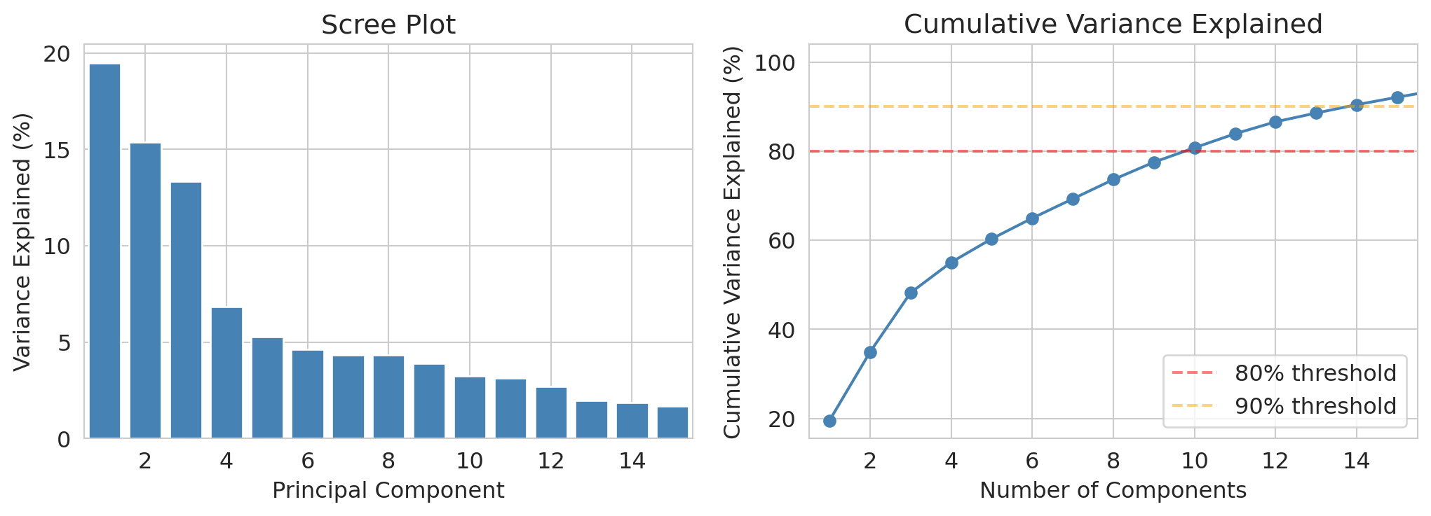
## The scree plot: how many components do we need?
The **scree plot** shows how much variance each PC explains. We look for an **elbow** — the point where adding more PCs doesn't help much. This heuristic is called the **elbow method**.
```{python}
# Scree plot: individual and cumulative variance explained
fig, axes = plt.subplots(1, 2, figsize=(11, 4))

axes[0].bar(range(1, len(pca.explained_variance_ratio_)+1),
            pca.explained_variance_ratio_ * 100,
            color='steelblue', edgecolor='white')
axes[0].set_xlabel('Principal component')
axes[0].set_ylabel('Variance explained (%)')
axes[0].set_title('Scree plot')
axes[0].set_xlim(0.5, 15.5)

cumvar = np.cumsum(pca.explained_variance_ratio_) * 100
axes[1].plot(range(1, len(cumvar)+1), cumvar, 'o-', color='steelblue')
axes[1].axhline(y=80, color='red', linestyle='--', alpha=0.5, label='80% threshold')
axes[1].axhline(y=90, color='orange', linestyle='--', alpha=0.5, label='90% threshold')
axes[1].set_xlabel('Number of Components')
axes[1].set_ylabel('Cumulative variance explained (%)')
axes[1].set_title('Cumulative variance explained')
axes[1].legend()
axes[1].set_xlim(0.5, 15.5)

plt.tight_layout()
plt.show()
```
How many PCs do we need to reach common variance thresholds?
```{python}
# How many PCs for various thresholds?
for threshold in [0.7, 0.8, 0.9]:
    n_needed = np.argmax(cumvar >= threshold*100) + 1
    print(f"  {threshold*100:.0f}% variance: need {n_needed} PCs (out of {len(numeric_cols)})")
```
We need about 8-10 PCs to capture 70-80% of the variance, or 14 to reach 90%. That's a big reduction from 23 columns — but not as dramatic as "just 5 PCs capture everything." Real data is messy, and the variance is spread out.
Still, the first few PCs do capture meaningful structure. Let's interpret them.
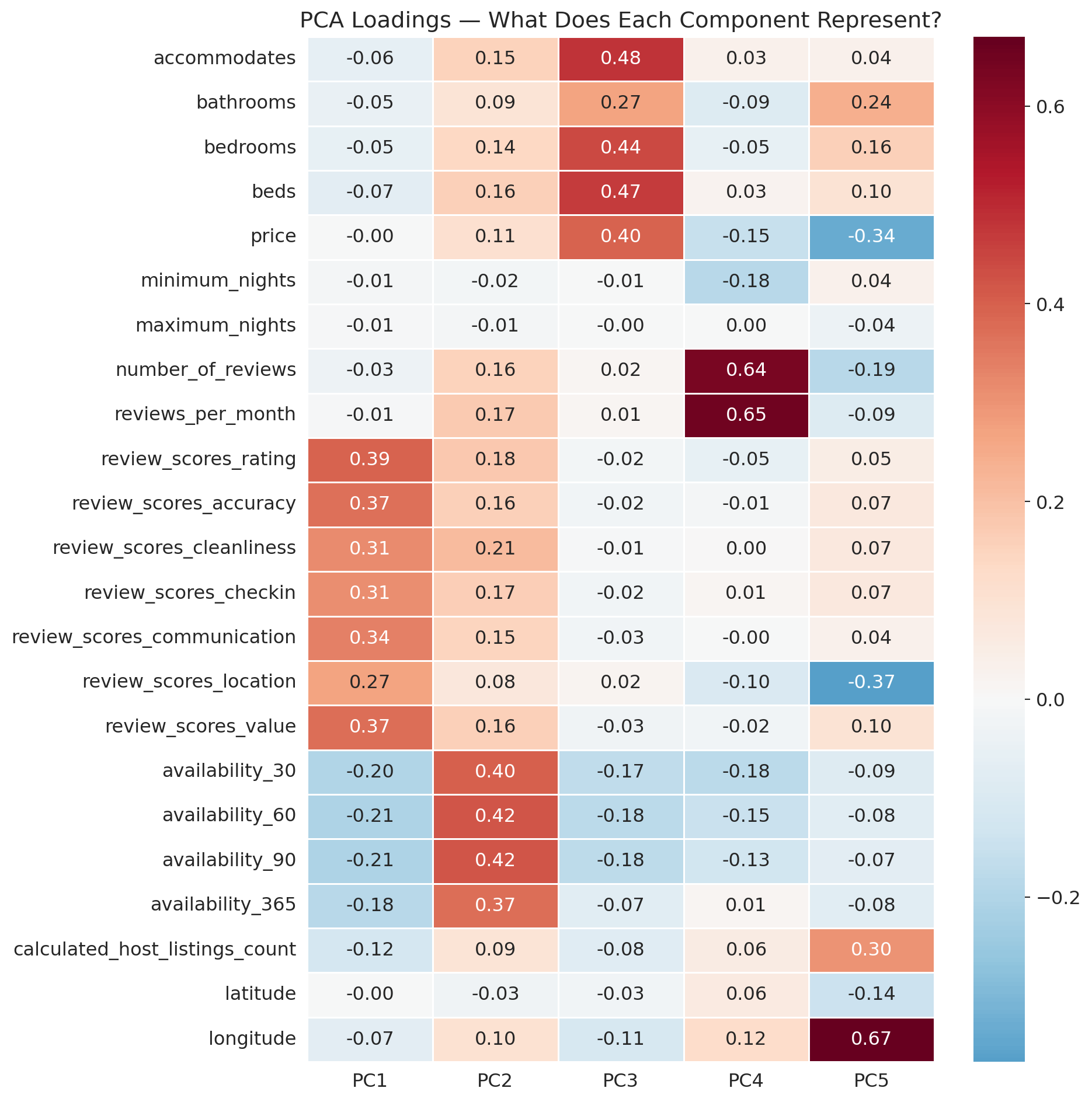
## Interpreting the principal components
Each PC is a weighted combination of the original features. The **loadings** — the weights — tell us what each PC represents.
:::{.callout-tip}
## Think about it
Now that we've standardized, what groupings of features do you expect PCA to find? Think about which Airbnb features tend to be correlated with each other.
:::
```{python}
# PC loadings heatmap for first 5 PCs
loadings = pd.DataFrame(
    pca.components_[:5].T,
    index=numeric_cols,
    columns=[f'PC{i+1}' for i in range(5)]
)

fig, ax = plt.subplots(figsize=(10, 10))
sns.heatmap(loadings, annot=True, fmt='.2f', cmap='RdBu_r', center=0,
            ax=ax, linewidths=0.5)
ax.set_title('PCA loadings — what does each component represent?')
plt.tight_layout()
plt.show()
```
Let's look at the strongest contributors to PC1 and PC2.
```{python}
# Interpret PC1: show top positive and negative loadings
print("PC1: Top loadings")
pc1 = loadings['PC1'].sort_values()
print("  Most negative:")
for feat, val in pc1.head(3).items():
    print(f"    {feat:>35s}: {val:+.3f}")
print("  Most positive:")
for feat, val in pc1.tail(3).items():
    print(f"    {feat:>35s}: {val:+.3f}")
```
Now PC2:
```{python}
print("PC2: Top loadings")
pc2 = loadings['PC2'].sort_values()
print("  Most negative:")
for feat, val in pc2.head(3).items():
    print(f"    {feat:>35s}: {val:+.3f}")
print("  Most positive:")
for feat, val in pc2.tail(3).items():
    print(f"    {feat:>35s}: {val:+.3f}")
```
**Telling the story of each PC:**
- **PC1** contrasts review scores (positive: rating, value, accuracy) against availability windows (negative: availability_30, _60, _90). Listings that score high on PC1 have strong reviews but low availability — popular, booked-up places. Listings that score low on PC1 have lots of open dates but weaker reviews.
- **PC2** loads heavily on availability_30, _60, and _90 (all positive), with weak negative loadings on latitude, minimum_nights, and maximum_nights. This component captures a "calendar openness" factor — listings with many available dates in the near term score high on PC2, regardless of review quality.
Notice how PCA automatically discovered these natural groupings. We didn't tell it about "review quality" or "calendar availability" — it found these dimensions by following the variance.
### Tracing one listing through PCA
Let's pick one listing and trace it through the entire PCA pipeline. This exercise makes the loadings concrete.
```{python}
# Pick a listing and show its original features and PC scores
example_idx = df.index[0]
example_features = df.loc[example_idx]
example_scores = scores[0]

print(f"Listing #{example_idx}:")
print(f"\nOriginal features (a few):")
for col in ['accommodates', 'bedrooms', 'review_scores_rating',
            'review_scores_cleanliness', 'price']:
    print(f"  {col:>30s}: {example_features[col]:>8.1f}")
print(f"\nPC scores:")
for i in range(3):
    print(f"  PC{i+1}: {example_scores[i]:+.2f}")
```
What do those scores tell us about this listing?
```{python}
# What does this listing's PC1 score mean?
print("PC1 is the 'popular & booked-up' factor (high reviews, low availability).")
print(f"This listing's PC1 score = {example_scores[0]:+.2f}")
if example_scores[0] > 0:
    print("  → Positive: strong reviews, limited availability.")
else:
    print("  → Negative: weaker reviews or lots of open dates.")
print(f"\nPC2 is the 'calendar openness' factor (high near-term availability).")
print(f"This listing's PC2 score = {example_scores[1]:+.2f}")
if example_scores[1] > 0:
    print("  → Positive: many available dates in the next 30-90 days.")
else:
    print("  → Negative: fewer available dates in the near term.")
```
## The math behind PCA: SVD
To understand what the SVD produces, two definitions from linear algebra are needed. These definitions build on the vector and span concepts from Chapter 4.
:::{.callout-important}
## Definition: Basis and orthonormal basis
A **basis** for a subspace is a minimal set of linearly independent vectors that spans it. The number of vectors in any basis equals the **dimension** of the subspace.
An **orthonormal basis** is a basis where every vector has norm 1 and every pair of vectors is orthogonal (inner product = 0). Orthonormal bases are especially convenient: to find the coordinates of a point, you just take dot products — no matrix inversion needed. PCA finds an orthonormal basis aligned with the directions of maximum variance.
:::
Now that you've seen PCA work, let's look under the hood. PCA is powered by the **SVD** (**Singular Value Decomposition**). The assigned reading (VanderPlas Ch 5.09) covers the sklearn implementation. If you've taken EE103, see VMLS Chapter 16 for a deeper treatment.
The exact SVD of the standardized (centered and scaled) data matrix is:
$$X = U S V^T$$
PCA keeps only the first $k$ components, giving a rank-$k$ approximation:
$$X \approx U_k S_k V_k^T$$
- The columns of $V$ are the **principal component directions** (the new axes)
- The diagonal of $S$ contains the **singular values** — the fraction of total variance captured by PC$i$ is $\sigma_i^2 / \sum_j \sigma_j^2$
- The rows of $US$ are the **PC scores** — row $i$ gives listing $i$'s coordinates in the new basis
:::{.callout-important}
## Definition: Eckart-Young-Mirsky theorem
Among all rank-$k$ approximations to $X$, the truncated SVD has the smallest total squared error (Frobenius norm). No other $k$-dimensional summary can do better.
:::
## PCA as regression onto optimal covariates
Here's the key insight that connects PCA to everything we've learned.
In regression (Chapter 5), we had a fixed set of features $X$ and found the best weights $w$ to minimize $\|y - Xw\|^2$. We chose the features; the math found the coefficients.
PCA is the same optimization, except we also get to choose $X$. We're minimizing $\|Y - XW\|_F^2$ over *both* the scores $X$ ($= U_k S_k$) and the directions $W$ ($= V_k^T$) simultaneously. PCA finds the best covariates AND the best coefficients.
These two views — maximizing variance captured and minimizing reconstruction error — are mathematically equivalent. This equivalence explains why PCA feels like a natural extension of regression: it IS regression, but with the freedom to pick the best possible features.
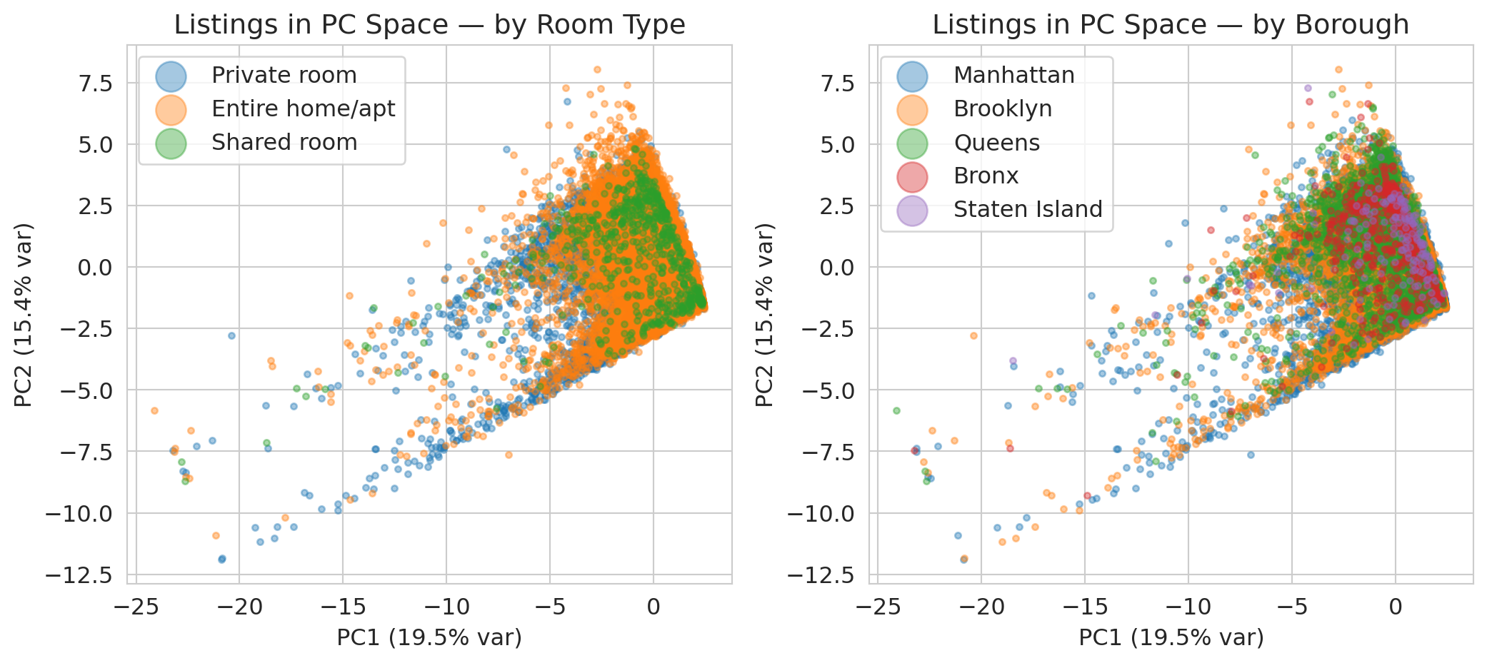
## Biplot: visualizing listings in PC space
Let's project every listing into the first two PCs and see if patterns emerge. We'll color by room type to see if PCA captures that distinction.
```{python}
# Create a dataframe with PC scores and metadata
# Use neighbourhood_group_cleansed (or neighbourhood_group as fallback)
borough_col = ('neighbourhood_group_cleansed'
               if 'neighbourhood_group_cleansed' in airbnb.columns
               else 'neighbourhood_group')

plot_df = pd.DataFrame({
    'PC1': scores[:, 0],
    'PC2': scores[:, 1],
    'room_type': airbnb.loc[df.index, 'room_type'].values,
    'borough': airbnb.loc[df.index, borough_col].values
})
```
Let's plot every listing in PC space, coloring by room type and borough.
```{python}
fig, axes = plt.subplots(1, 2, figsize=(11, 5))

# Color by room type
for rt in plot_df['room_type'].unique():
    mask = plot_df['room_type'] == rt
    axes[0].scatter(plot_df.loc[mask, 'PC1'], plot_df.loc[mask, 'PC2'],
                    alpha=0.4, s=10, label=rt)
axes[0].set_xlabel(f"PC1 ({pca.explained_variance_ratio_[0]*100:.1f}% var)")
axes[0].set_ylabel(f"PC2 ({pca.explained_variance_ratio_[1]*100:.1f}% var)")
axes[0].set_title('Listings in PC space — by room type')
axes[0].legend(markerscale=5)

# Color by borough
for b in ['Manhattan', 'Brooklyn', 'Queens', 'Bronx', 'Staten Island']:
    mask = plot_df['borough'] == b
    axes[1].scatter(plot_df.loc[mask, 'PC1'], plot_df.loc[mask, 'PC2'],
                    alpha=0.4, s=10, label=b)
axes[1].set_xlabel(f"PC1 ({pca.explained_variance_ratio_[0]*100:.1f}% var)")
axes[1].set_ylabel(f"PC2 ({pca.explained_variance_ratio_[1]*100:.1f}% var)")
axes[1].set_title('Listings in PC Space — by Borough')
axes[1].legend(markerscale=5)

plt.tight_layout()
plt.show()
```
Room types show some separation along the first two PCs, but there's a lot of overlap — PCA captures broad trends, not clean clusters.
Boroughs show less separation in these first two PCs. Geography isn't the dominant source of variance in the standardized data — review patterns and availability matter more.
## PCA vs. feature selection
:::{.callout-tip}
## Think about it
Couldn't we just pick the 5 most important features instead of doing PCA? When would PCA be better than, say, Lasso (Chapter 6)?
:::
PCA creates *new* features that are combinations of the originals — it's **dimensionality reduction**. Lasso picks a subset of existing features — that's **feature selection**. PCA is especially useful when your original features are correlated (like the six review scores): it creates uncorrelated summaries that capture more information per component.
A common downstream use of PCA is to feed the top-$k$ PC scores into a clustering algorithm — Euclidean distances are more trustworthy in the reduced space than in the raw features. See [Chapter 15](lec15-clustering.qmd) for the Tabula Muris single-cell atlas, the marquee published example of this PCA-then-cluster recipe.
:::{.callout-warning}
## PCA on mixed data
We only used numeric columns. PCA requires numeric input — if you one-hot encode categoricals and run PCA, you're mixing binary (0/1) columns with continuous columns. The geometry of binary data is very different (all points land on vertices of a hypercube), so standard PCA doesn't handle this well.
For this course, just use the numeric columns. If you're curious about mixed data, look up Multiple Correspondence Analysis — but that's beyond our scope.
:::
## Key takeaways
- **PCA finds the directions of maximum variance** in your data. Each principal component is a weighted combination of the original features.
- **The scree plot** tells you how many PCs you need. Look for an elbow — but don't expect a sharp one with real data.
- **Interpret the components.** PCA is not just a dimensionality reduction button — the loadings tell you *what* each component represents. Tell the story.
- **Always standardize first.** Without standardization, PCA is dominated by whichever feature has the largest scale.
- **PCA finds the best *linear* summary.** If your data lies on a curved surface or has complex cluster shapes, PCA's linear approximation may miss important structure.
## Coming up next
In **Chapter 15**, we'll move from summarizing data to *grouping* data. **K-means clustering** will discover modern NBA archetypes that cut across traditional positions — and then we'll look at four published case studies (cells, asthma, depression, stars) that turn on the same point: feature choice determines what the algorithm finds, and validation has to come from outside the clustering itself. PCA and k-means are cousins: same optimization framework, different constraints.
## Study guide
### Key ideas
- **PCA (Principal Component Analysis)** finds the directions of maximum variance in high-dimensional data, producing a lower-dimensional summary.
- **Principal component**: a new axis (direction) found by PCA. Each PC is a weighted combination of the original features.
- **Loading**: the weight of an original feature in a principal component. High loadings tell you which features drive that PC.
- **SVD (Singular Value Decomposition)**: the matrix factorization $X = USV^T$ that powers PCA. The columns of $V$ are the PC directions, the diagonal of $S$ holds the singular values, and the rows of $US$ give the PC scores.
- **Singular value**: the $i$-th diagonal entry of $S$. Its square is proportional to the variance explained by PC$i$.
- **Explained variance ratio**: the fraction of total variance captured by a given PC. Sum of all ratios = 1.
- **Scree plot**: bar chart of explained variance by component, used to decide how many PCs to keep.
- **Elbow method**: choosing the number of PCs at the "elbow" where the scree plot levels off.
- **Standardization (z-score)**: subtracting the mean and dividing by the standard deviation so all features have mean 0 and variance 1.
- PCA finds the best low-dimensional linear summary of your data by maximizing captured variance (equivalently, minimizing reconstruction error).
- PCA is regression where you also get to choose the features — it finds the optimal covariates AND coefficients simultaneously.
- Always standardize before PCA, or the result is dominated by whichever column has the biggest numbers.
- The Eckart-Young-Mirsky theorem guarantees that the SVD gives the best rank-$k$ approximation — no other $k$-dimensional summary can do better.
- PCA creates new combined features (dimensionality reduction), while Lasso selects a subset of existing features (feature selection).
### Computational tools
- `StandardScaler()` — standardizes features to mean 0 and variance 1
- `PCA()` — creates a PCA model; use `PCA(n_components=k)` to keep only $k$ components
- `.fit_transform(X)` — fit the model and transform the data in one step
- `.explained_variance_ratio_` — array of variance fractions for each PC
- `.components_` — matrix of loadings (each row is a PC, each column is a feature)
### For the quiz
- Know what standardization does and why it matters for PCA (covariance vs. correlation matrix).
- Be able to read a scree plot and estimate how many PCs capture a given fraction of variance.
- Be able to interpret loadings: given a loadings table, describe what a PC represents in plain language.
- Understand the difference between PCA (dimensionality reduction) and Lasso (feature selection).
- Know the Eckart-Young-Mirsky theorem by name: SVD gives the best rank-$k$ approximation.