---
title: "Hypothesis Testing Framework"
execute:
enabled: true
jupyter: python3
---
```{python}
import numpy as np
import pandas as pd
import matplotlib.pyplot as plt
import seaborn as sns
from scipy import stats
from scipy.stats import norm
import warnings
warnings.filterwarnings('ignore')
sns.set_style('whitegrid')
plt.rcParams['figure.figsize'] = (7, 4.5)
plt.rcParams['font.size'] = 12

DATA_DIR = 'data'
np.random.seed(42)
```
In [Chapter 9](lec09-permutation-tests.qmd) we shuffled labels in the ACTG 175 data and read off a p-value of about $10^{-4}$. By 2026 standards the verdict was easy: the drug worked. But in 1991, the trial *hadn't been run yet*, and the people designing it faced a different set of questions:
- **How many patients should we enroll?** Too few and we miss a real effect; too many wastes money and exposes more people than necessary to an experimental regimen.
- **How small a p-value is convincing?** The FDA had to commit to a threshold *before* the data came in.
- **What kinds of mistakes are we willing to make, and at what rate?**
Chapter 9 framed hypothesis testing as a question you ask *of data you already have*, leaving these on the table. This chapter takes the prospective view: hypothesis testing as a tool for **designing a study**. Three new ideas make that possible:
1. A formal accounting of the **two errors** a test can make, and the rates at which they occur.
2. A **formula-based** test (Welch's t-test) whose math we can solve before any data exists. Permutation tests need data to shuffle; we don't have data yet.
3. **Power analysis**, which uses that math to size a study — once we are willing to *guess* what effect we hope to detect.
We close by reconciling Chapter 8's bootstrap CI with the hypothesis test (they say the same thing) and by examining a failure mode of large studies: any nonzero effect eventually becomes "significant," whether it matters or not.
Notation: $H_0$ for the null, $H_1$ for the alternative, $p$ for the p-value, $\alpha$ for the significance threshold. Chapter 9 defined $H_0$ and the p-value informally; we formalize them here and add a careful definition of $H_1$, which we'll need to talk about errors and power.
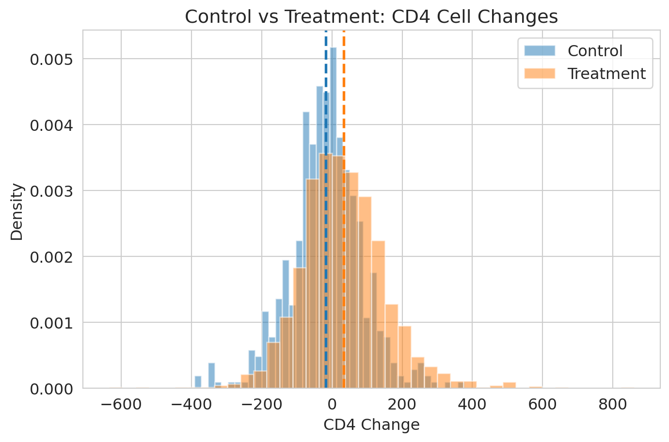
```{python}
df = pd.read_csv(f'{DATA_DIR}/clinical-trial/ACTG175.csv')
df['cd4_change'] = df['cd420'] - df['cd40']
control = df[df['treat'] == 0]['cd4_change'].dropna()
treatment = df[df['treat'] == 1]['cd4_change'].dropna()
observed_effect = treatment.mean() - control.mean()
print(f"ACTG 175: control n={len(control)}, treatment n={len(treatment)}")
print(f"Observed treatment effect: {observed_effect:.1f} CD4 cells")
```
## The framework in four lines
Every hypothesis test follows the same recipe:
1. **State $H_0$ and $H_1$** — the competing claims about the world.
2. **Pick a test statistic** — one number that summarizes the evidence.
3. **Determine the null distribution** — what the test statistic looks like if $H_0$ were true. (Chapter 9: by shuffling. This chapter: by formula.)
4. **Compute the p-value** — and reject $H_0$ when $p < \alpha$.
For ACTG 175:
| | |
|--|--|
| **$H_0$** | The combination treatment has no effect on CD4 change. |
| **$H_1$** | It does (effect $\neq 0$). |
| **Test statistic** | Difference in group means, scaled by its standard error — the **t-statistic** below. |
| **Null distribution** | Approximately Student's $t$ (justified by the CLT). |
| **p-value** | Probability of a t-statistic at least this extreme if $H_0$ were true. |
What's new in this chapter is row 3 — a formula-based null distribution — and a more precise vocabulary for the decision rule that uses it.
::: {.callout-important}
## Definition: null and alternative hypotheses
The **null hypothesis** $H_0$ is a single, specific claim about the world — typically "no effect" or "no difference" — that the test tries to disprove. For ACTG: $H_0: \mu_T - \mu_C = 0$ (the population mean CD4 change is the same in the two arms).
The **alternative hypothesis** $H_1$ is the *complement* of $H_0$ within the model: every state of the world that $H_0$ rules out. For ACTG: $H_1: \mu_T - \mu_C \neq 0$ (two-sided) or $H_1: \mu_T - \mu_C > 0$ (one-sided, if only beneficial effects are of interest).
A hypothesis test does *not* require us to commit to any particular value of the effect inside $H_1$. We just ask whether the data are surprising enough under $H_0$ to rule it out. The test works without committing to a specific effect size.
The catch — which we develop in this chapter — is that $H_1$ is a whole **family** of possible worlds (all the nonzero effects), not a single one. Talking about Type II error or power forces us to pick a specific effect inside $H_1$: the chance of detecting a real effect depends on how big it is.
:::
## Two errors, not one
Until now we have spoken as if the only worry was rejecting $H_0$ when it's true. There is a symmetric worry: failing to reject $H_0$ when $H_1$ is true.
Think of a courtroom. $H_0$ is "innocent until proven guilty."
- **Type I error** = convicting an innocent person. We rejected $H_0$ when it was true. *In the trial: approving a useless drug.*
- **Type II error** = letting a guilty person go free. We failed to reject $H_0$ when $H_1$ was true. *In the trial: rejecting a drug that saves lives.*
| | $H_0$ true (no effect) | $H_1$ true (real effect) |
|--|---|---|
| **Reject $H_0$** | Type I error (rate $\alpha$) | Correct |
| **Fail to reject $H_0$** | Correct | Type II error (rate $\beta$) |
::: {.callout-important}
## Definition: significance level and the two error rates
- **Significance level** $\alpha$: the threshold at which we reject $H_0$. By construction, $P(\text{reject } H_0 \mid H_0 \text{ true}) = \alpha$ — the **Type I error rate**.
- **Type II error rate** $\beta$: $P(\text{fail to reject } H_0 \mid H_1 \text{ true})$.
We'll define **power** in the design section, where it does its work.
:::
::: {.callout-important}
## "Fail to reject" — not "accept"
A non-significant result means the data are compatible with $H_0$ — but they may also be compatible with many other hypotheses. Absence of evidence is not evidence of absence. As Einstein (reportedly) put it: *"No amount of experimentation can ever prove me right; a single experiment can prove me wrong."*
:::
The two error rates trade off as we move the rejection threshold. Picture the test statistic's distribution under $H_0$ (centered at zero) and under a specific $H_1$ (shifted). Anything past the threshold counts as "reject."
::: {.callout-tip}
## Think about it
Before scrolling: if we move the rejection threshold *to the right* (stricter $\alpha$ — harder to reject), what happens to the false-positive region under $H_0$? To the false-negative region under $H_1$? Predict before you read on.
:::
```{python}
sigma = control.std()
n_per = len(control)
se = sigma * np.sqrt(2 / n_per)
illustrative_effect = 1.0 * se   # small effect so both tails are visible

x = np.linspace(-4*se, illustrative_effect + 4*se, 500)
null_dist = norm.pdf(x, 0, se)
alt_dist  = norm.pdf(x, illustrative_effect, se)
cutoff = norm.ppf(1 - 0.05, 0, se)   # one-sided α = 0.05 for visual clarity

fig, ax = plt.subplots(figsize=(9, 4.5))
ax.plot(x, null_dist, 'b-', lw=2, label='Null ($H_0$: no effect)')
ax.plot(x, alt_dist,  'r-', lw=2, label=f'Alternative ($H_1$: real effect)')
ax.fill_between(x[x >= cutoff], null_dist[x >= cutoff], alpha=0.3, color='blue',
                label='Type I error rate ($\\alpha$)')
ax.fill_between(x[x <= cutoff], alt_dist[x <= cutoff],  alpha=0.3, color='red',
                label='Type II error rate ($\\beta$)')
ax.axvline(cutoff, color='gray', ls='--', lw=1.5, label='Rejection threshold')
ax.set_xlabel('Test statistic')
ax.set_ylabel('Density')
ax.set_title('One-sided test: $\\alpha$ and $\\beta$ are areas under different curves')
ax.legend(fontsize=9, loc='upper right')
plt.show()
```
The picture makes one asymmetry visible. We **control $\alpha$ directly** — it's just where we draw the threshold. We do **not** control $\beta$ directly: the size of the red region depends on how far the alternative distribution is shifted, i.e. on the *true* effect size, which we don't know. Power analysis (later in this chapter) computes $\beta$ *given* an assumed effect size, but the assumption is unavoidable.
Moving the threshold right (stricter $\alpha$) shrinks the blue region but grows the red region. There is no free lunch — only a *choice* of which error you'd rather make more often.
The convention $\alpha = 0.05$ is from R.A. Fisher's 1925 textbook: he called it a "convenient" threshold and it stuck. There is nothing magical about it. Particle physics uses roughly $0.0000003$; the FDA effectively uses $0.05^2 \approx 0.0025$ by requiring two independent positive trials. Once we work out power, we'll come back to what $\alpha$ should be for a given decision.
## From simulation to formula: Welch's t-test
In Chapter 9, we built the null distribution by shuffling labels — 10,000 fake datasets, each producing one fake test statistic. That answers "is the effect real?" for *this* dataset. But it can't answer the design question — *if I enroll 200 patients per arm and the true effect is 30 CD4 cells, how often will I reject?* — because there is no data to shuffle. We need a closed-form expression for the null distribution.
The closed-form alternative was worked out a century before electronic computers — at a brewery, by someone facing exactly this problem in miniature. In 1908, William Sealy Gosset, a chemist at the Guinness brewery in Dublin, needed to compare barley varieties and yeast strains with only a handful of samples per batch. The normal approximation was unreliable at $n = 5$ or $10$, and he could not bootstrap or simulate — those tools were decades from existing. So he derived analytically the exact distribution of the sample mean divided by its standard deviation. He published in 1908 under the pseudonym "Student" — Guinness forbade employees from publishing under their real names, fearing competitors would learn they were using statistics. (See Salsburg, *The Lady Tasting Tea*, Ch. 2.) The result is what we now call **Student's $t$-distribution**.
### What does the t distribution look like?
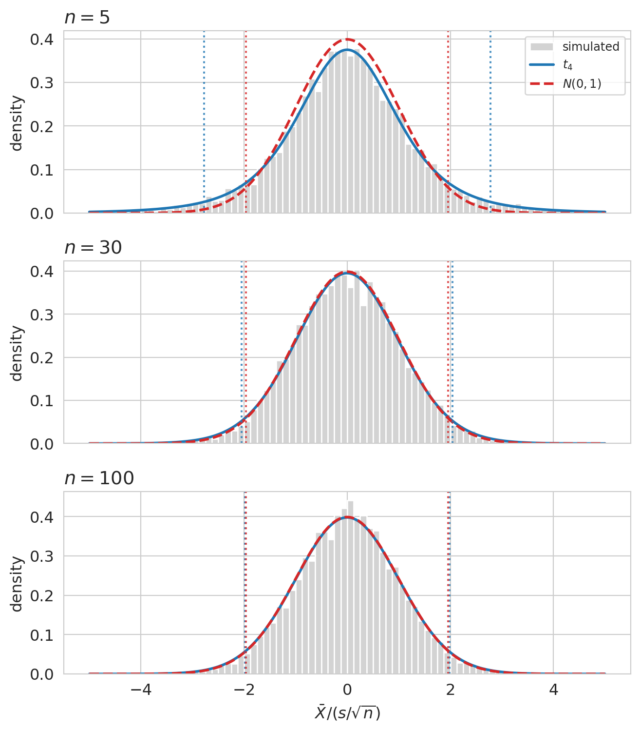
Before we bolt the formula onto a two-sample test, pause to look at the distribution Gosset derived. If his analytical work is right, the studentized statistic $\bar X / (s/\sqrt n)$ — computed on samples drawn from a known $N(0, 1)$ population — should match $t_{n-1}$ exactly, and converge to $N(0, 1)$ as $n$ grows.
```{python}
n_reps = 10_000
sample_sizes = [5, 30, 100]
rng = np.random.default_rng(seed=42)

x = np.linspace(-5, 5, 400)
fig, axes = plt.subplots(3, 1, figsize=(7, 8), sharex=True)

for ax, n in zip(axes, sample_sizes):
    samples = rng.standard_normal(size=(n_reps, n))
    t_stats = samples.mean(axis=1) / (samples.std(axis=1, ddof=1) / np.sqrt(n))

    ax.hist(t_stats, bins=80, range=(-5, 5), density=True,
            color='lightgray', edgecolor='white', label='simulated')
    ax.plot(x, stats.t.pdf(x, df=n-1), color='C0', lw=2,
            label=f'$t_{{{n-1}}}$')
    ax.plot(x, stats.norm.pdf(x), color='C3', lw=2, ls='--',
            label='$N(0,1)$')

    t_cut = stats.t.ppf(0.975, df=n-1)
    z_cut = 1.96
    for c in (-t_cut, t_cut):
        ax.axvline(c, color='C0', ls=':', alpha=0.8)
    for c in (-z_cut, z_cut):
        ax.axvline(c, color='C3', ls=':', alpha=0.8)

    ax.set_title(f'$n = {n}$', loc='left')
    ax.set_ylabel('density')

axes[0].legend(loc='upper right', fontsize=9)
axes[-1].set_xlabel(r'$\bar X / (s/\sqrt{n})$')
plt.tight_layout()
plt.show()
```
At $n = 5$, the simulated histogram has visibly fatter tails than $N(0, 1)$, and Gosset's $t_4$ threads through the histogram exactly. The reason: $s$ is a noisy estimate of $\sigma$ when $n$ is small, so the denominator $s/\sqrt n$ varies more than $\sigma/\sqrt n$ would, and that extra variability fattens the ratio's tails. By $n = 30$, the studentized statistic and the normal are visually almost identical; by $n = 100$ they coincide for any practical purpose.
The dotted vertical lines mark the two-sided 5% cutoffs of each distribution. At $n = 5$ the t-cutoffs sit well outside the normal cutoffs at $\pm 1.96$ — using the normal cutoffs would over-reject under $H_0$. By $n = 100$ the cutoffs coincide. Gosset's correction matters precisely where the normal approximation is unreliable, and fades to nothing where it isn't.
### Welch's two-sample formula
The two-sample version — for "do these two groups have the same mean?" — is **Welch's t-test**, a refinement of Gosset's that drops the equal-variance assumption. Using the same notation as the Chapter 8 CLT — let $\bar X_T$, $\bar X_C$ be the **sample means** of the two groups, $s_T^2$, $s_C^2$ the **sample variances** (with the standard $n-1$ divisor), and $n_T$, $n_C$ the sample sizes — the test statistic is
$$t \;=\; \frac{\bar{X}_T - \bar{X}_C}{\sqrt{s_T^2/n_T \;+\; s_C^2/n_C}}.$$
The numerator is the observed effect (the same difference of sample means we bootstrapped in Chapter 8). The denominator is exactly the standard-error formula $\widehat{\text{SE}}$ from Chapter 8 — the plug-in estimate of the SD of $\bar X_T - \bar X_C$, with each variance divided by its own sample size and the two added (the groups are independent).
Under $H_0$ — and the CLT-style assumption that each group mean is approximately normal — $t$ has a known distribution (Student's $t$) that depends only on the sample sizes, not on the unknown population distribution. That known distribution is the engine of design analysis: we can compute it by formula for any $n_T, n_C$, no data required.
Two flavors of two-sample t-test exist. The original (Student's) assumes the two groups have equal variance; Welch's drops that assumption by adjusting the standard error and the degrees of freedom. In real data the variances are rarely equal, so Welch's is the safe default — `equal_var=False` in `scipy`. Use it unless you have a positive reason to assume equal variance.
Run Welch's on ACTG and compare to Chapter 9's permutation result:
```{python}
t_stat, p_value = stats.ttest_ind(treatment, control, equal_var=False)
print(f"Welch's t-test:    t = {t_stat:.2f},  p = {p_value:.2e}")
print("Permutation (Ch 9):                p ≈ 1×10⁻⁴ (limited by 10,000 shuffles)")
```
Both verdicts: $H_0$ rejected at any conventional $\alpha$. The advantage of the formula isn't a different answer on *this* data — it's that the formula will *also* tell us what would have happened with 100 patients per arm, or 30, or 1000.
::: {.callout-tip}
## The same machinery, in tech: A/B testing
The dominant industrial application of two-sample comparison is **A/B testing**. A growth team at a streaming company runs a two-week test on a new homepage. Variant B converts at 4.2% ($n = 12{,}400$); variant A at 4.0% ($n = 12{,}200$). The same Welch's logic — observed difference divided by its standard error, p-value from the $t$-distribution — yields $p \approx 0.04$. Identical recipe to the clinical trial; only the stakes change.
Type I error here: ship a feature that doesn't actually help (development cost, maintenance burden). Type II error: kill a feature that would have moved the needle. Most companies set a *less strict* $\alpha$ than the FDA — a wrong shipping decision is reversible, and shipping faster has its own value. The cost ratio of the two errors should set $\alpha$ in any setting; the FDA and a startup land on different points of the same curve.
:::
::: {.callout-note collapse="true"}
## Going deeper: when the formula and the shuffle disagree
The t-test relies on the two sample means being approximately normal. Under exact normality of the underlying data, this is automatic; otherwise the CLT does the work, and the test's p-value is approximate. With ACTG's $n \approx 1000$ per arm and finite-variance outcomes, the approximation holds easily. With small or heavy-tailed samples (financial returns, rare-event counts), the CLT may not have kicked in; the t-test's stated p-value can then be off by enough to flip the decision. The permutation test only requires exchangeability under the null, so it remains valid where the t-test fails. **Rule of thumb:** prefer the t-test for $n > 30$ per arm with roughly symmetric data; reach for permutation when either condition fails.
:::
## Verifying $\alpha$ controls Type I error
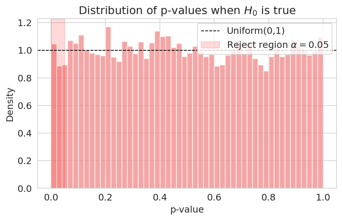
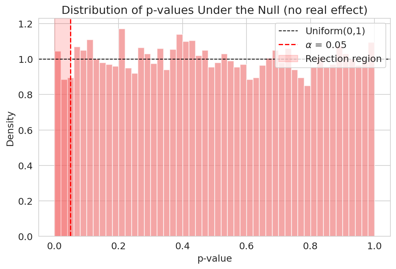
Welch's t-test rejected the null hypothesis decisively on ACTG. Before we trust it for design, let's confirm the other half of the contract: when $H_0$ is *true*, the test should reject only $\alpha$ of the time. Take the ACTG **control group only** — no treatment effect can possibly exist within it — split it randomly in half, and run Welch's t-test. Any rejection is a false positive. Repeat 10,000 times.
```{python}
control_vals = control.values
n_sims = 10_000
p_values_null = np.empty(n_sims)
for i in range(n_sims):
    s = np.random.permutation(control_vals)
    half = len(s) // 2
    _, p_values_null[i] = stats.ttest_ind(s[:half], s[half:], equal_var=False)

print(f"Fraction p < 0.05: {np.mean(p_values_null < 0.05):.3f}  (target 0.05)")
print(f"Fraction p < 0.01: {np.mean(p_values_null < 0.01):.3f}  (target 0.01)")
print(f"Fraction p < 0.10: {np.mean(p_values_null < 0.10):.3f}  (target 0.10)")
```
```{python}
fig, ax = plt.subplots(figsize=(7, 4))
ax.hist(p_values_null, bins=50, density=True, color='lightcoral', alpha=0.7, edgecolor='white')
ax.axhline(1.0, color='black', ls='--', lw=1, label='Uniform(0,1)')
ax.axvspan(0, 0.05, alpha=0.15, color='red', label='Reject region $\\alpha=0.05$')
ax.set_xlabel('p-value'); ax.set_ylabel('Density')
ax.set_title('Distribution of p-values when $H_0$ is true')
ax.legend()
plt.show()
```
Under the null, p-values from a correctly specified test are **Uniform(0, 1)** — the flat density on $[0,1]$ from your probability course. Choosing $\alpha = 0.05$ therefore rejects exactly 5% of the time when $H_0$ is true: 5% of uniform draws fall below 0.05. The uniformity is exact for *exact* tests (e.g., the permutation test of Chapter 9 with all permutations); for Welch's t-test it's approximate, with the approximation getting better as $n$ grows. Either way, on this large dataset, $\alpha$ does what it advertises.
The other error — Type II — is harder to characterize. It depends not just on $\alpha$, but on how big the true effect is.
## Power: how many patients do we need?
Recall that $H_1$ is a *family* of possible worlds — every nonzero effect lives in it. A p-value asks "are the data surprising under $H_0$?" without committing to any particular alternative. **Power can't.** To compute power we must pick one specific point inside $H_1$ — the effect we hope to detect. That commitment is what distinguishes design analysis from p-value computation.
::: {.callout-important}
## Definition: power
$$
\text{Power} \;:=\; 1 - \beta \;=\; P(\text{reject } H_0 \mid \text{true effect} = \Delta).
$$
The probability of correctly detecting a real effect of size $\Delta$, when $\Delta$ is the true effect.
:::
Suppose we are planning a new HIV trial and we believe the experimental arm could shift mean CD4 change by **30 cells** relative to control. How many patients do we need so that, *if* the true effect really is 30, the test will detect it most of the time?
The **power calculation** is the inverse of the question we have been asking. So far: given data, what's the p-value? Now: given a hoped-for effect, what's the chance of a small p-value?
::: {.callout-warning}
## Power analysis requires you to **guess the effect size**
You cannot do a power analysis without committing to an effect size. Recall that $H_1: \mu_T - \mu_C \neq 0$ is a *family* of possible worlds — small effects, medium effects, large effects all live inside it, each with its own power. To compute one number, we have to pick one specific point in $H_1$ — typically called the **detectable effect** $\Delta$. Where that guess comes from:
- **Prior studies** of similar interventions (most defensible).
- **The smallest effect that would matter** clinically or commercially — the "minimum detectable effect" you care about distinguishing from zero.
- **A pilot study** designed specifically to estimate plausible effect sizes.
The guess is unavoidable, and it dominates the answer: doubling the assumed effect size cuts the required sample size by roughly a factor of four. Power analyses in published trial protocols always include the assumed effect; reviewers always scrutinize it.
:::
What does picking an effect size mean? Each $\Delta$ corresponds to a different *world we might be in* — control patients drawn from one CD4-change distribution, treatment patients from a copy of that distribution shifted by $\Delta$. Bigger $\Delta$ means the two populations are farther apart and easier to tell apart from data; smaller $\Delta$ means the two populations overlap so heavily that any individual observation could plausibly come from either.
```{python}
sigma_pop = control.std()
mu_C = control.mean()
deltas = [0, 10, 30, 50]
colors_pop = ['black', 'tab:blue', 'tab:orange', 'tab:red']

x = np.linspace(mu_C - 3.5*sigma_pop, mu_C + 3.5*sigma_pop + 50, 500)

fig, ax = plt.subplots(figsize=(8, 4.5))
ax.plot(x, norm.pdf(x, mu_C, sigma_pop), color='black', lw=2,
        label='Control ($\\Delta = 0$)')
for delta, color in zip(deltas[1:], colors_pop[1:]):
    ax.plot(x, norm.pdf(x, mu_C + delta, sigma_pop), color=color, lw=2, ls='--',
            label=f'Treatment ($\\Delta = {delta}$)')

# Mark each mean on the x-axis
for delta, color in zip(deltas, colors_pop):
    ax.axvline(mu_C + delta, color=color, lw=0.8, alpha=0.4)

ax.set_xlabel('CD4 change (per patient)')
ax.set_ylabel('Density')
ax.set_title("Each $\\Delta$ in $H_1$ is a different world: how far apart are the two populations?")
ax.legend(loc='upper right', fontsize=10)
plt.show()
```
With $\sigma \approx 105$ CD4 cells of patient-to-patient variation, even a $\Delta = 50$ shift leaves the two distributions heavily overlapped — knowing one patient's CD4 change tells you almost nothing about which arm they were in. What rescues us is sample size: the *sampling distribution* of $\bar X_T - \bar X_C$ has SD $\sqrt{s_T^2/n_T + s_C^2/n_C}$, which shrinks as $n$ grows. Power is the chance that the *sample mean difference* falls past the rejection threshold under the assumed $\Delta$ — and that chance grows with both $\Delta$ and $n$.
We can compute power by simulation — same engine as the Chapter 9 permutation, just with a true effect baked in. We simulate from a normal distribution here for tractability; the actual CD4-change distribution is somewhat skewed, but the approximation is fine at this $n$.
::: {.callout-tip}
## Think about it
Suppose the true treatment effect really is 30 CD4 cells (a meaningful but not huge effect for HIV). With **100 patients per arm**, what fraction of trials would correctly reject $H_0$? 90%? 75%? 50%? Guess before you read on.
:::
```{python}
def simulate_power(true_effect, n_per_group, alpha=0.05, n_sims=2000):
    sigma = control.std()
    rejections = 0
    for _ in range(n_sims):
        a = np.random.normal(0, sigma, n_per_group)
        b = np.random.normal(true_effect, sigma, n_per_group)
        _, p = stats.ttest_ind(a, b, equal_var=False)
        rejections += (p < alpha)
    return rejections / n_sims

print(f"Assumed true effect = 30 CD4 cells, n = 100 per group")
print(f"Estimated power = {simulate_power(30, 100):.2f}")
```
A power of 0.5 means we'd correctly detect the effect only half the time. That's the definition of an underpowered study: you'd be flipping a coin. The conventional target is **80% power** — chosen by convention, like $\alpha = 0.05$, but now widely accepted.
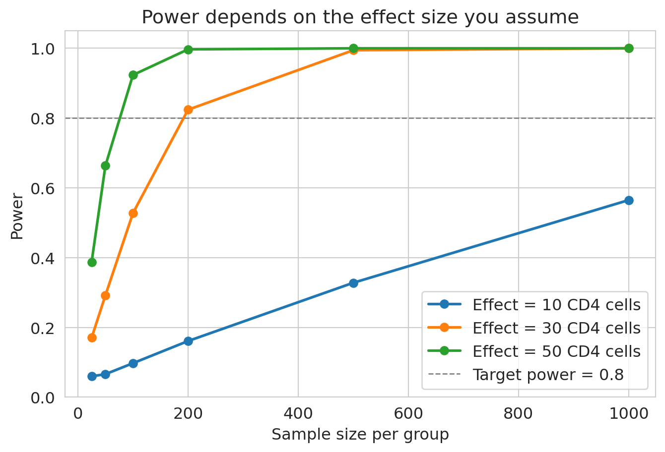
How does power vary with effect size and sample size? Vary both:
```{python}
# This cell takes ~15 seconds to run
sample_sizes = [25, 50, 100, 200, 500, 1000]
effect_sizes = [10, 30, 50]

fig, ax = plt.subplots(figsize=(8, 5))
for effect in effect_sizes:
    powers = [simulate_power(effect, n) for n in sample_sizes]
    ax.plot(sample_sizes, powers, 'o-', lw=2, label=f'Effect = {effect} CD4 cells')
ax.axhline(0.8, color='gray', ls='--', lw=1, label='Target power = 0.8')
ax.set_xlabel('Sample size per group'); ax.set_ylabel('Power')
ax.set_title('Power depends on the effect size you assume')
ax.legend(); ax.set_ylim(0, 1.05)
plt.show()
```
The curves quantify the design tradeoff: the smaller the effect we want to detect, the more patients we need — and the curve is far from linear. Going from "detect 50-cell effects" to "detect 10-cell effects" pushes required $n$ up by more than 25×.
In practice you'd skip the simulation and use the analytical formula, which `statsmodels` packages neatly. Effect sizes are reported as **Cohen's $d = \Delta / \sigma$**, where $\Delta$ is the assumed mean difference and $\sigma$ is the (assumed common) population SD — the effect in standard-deviation units, so the answer doesn't depend on the original units. Conventional shorthand: $d = 0.2$ small, $0.5$ medium, $0.8$ large.
```{python}
from statsmodels.stats.power import TTestIndPower
power_analysis = TTestIndPower()

d_assumed = 30 / control.std()
n_needed = power_analysis.solve_power(effect_size=d_assumed, power=0.8, alpha=0.05)
print(f"Assumed effect = 30 CD4 cells (Cohen's d = {d_assumed:.2f})")
print(f"  → need {n_needed:.0f} patients per group, {2*n_needed:.0f} total")
```
```{python}
d_actual = observed_effect / control.std()
power_actual = power_analysis.solve_power(effect_size=d_actual, nobs1=len(control), alpha=0.05)
print(f"ACTG 175 actually saw effect = {observed_effect:.1f} cells (d = {d_actual:.2f})")
print(f"  with n = {len(control)} per group → power = {power_actual:.4f}")
print(f"  (Far above 80% — they had more than enough patients for this effect.)")
```
::: {.callout-note}
## The power formula assumes more than the test does
`TTestIndPower` assumes both groups are normal with equal standard deviation. Welch's t-test itself works fine without that — but the **power formula** depends on knowing the variance, so power analyses inherit assumptions that the post-hoc test does not. If you suspect heavy tails or unequal variances, simulate power directly with the data-generating process you believe, as `simulate_power` does above.
:::
## What should $\alpha$ be?
We now have the mechanics: $\alpha$ controls Type I error, power controls Type II, and to compute power we have to commit to an effect size. The remaining design choice is $\alpha$ itself.
You're the FDA. Approving a useless \$1.3B drug exposes patients to side effects with no upside and burns billions in healthcare costs (Type I). Rejecting a drug that works denies treatment to people who would have benefited — and possibly survived (Type II). The cost ratio of those two errors is what should set $\alpha$, not convention.
::: {.callout-tip}
## Think about it
A drug might save 1,000 lives per year but costs \$2B to manufacture. What false positive rate would you accept? How does your answer change if the side-effect profile is severe?
:::
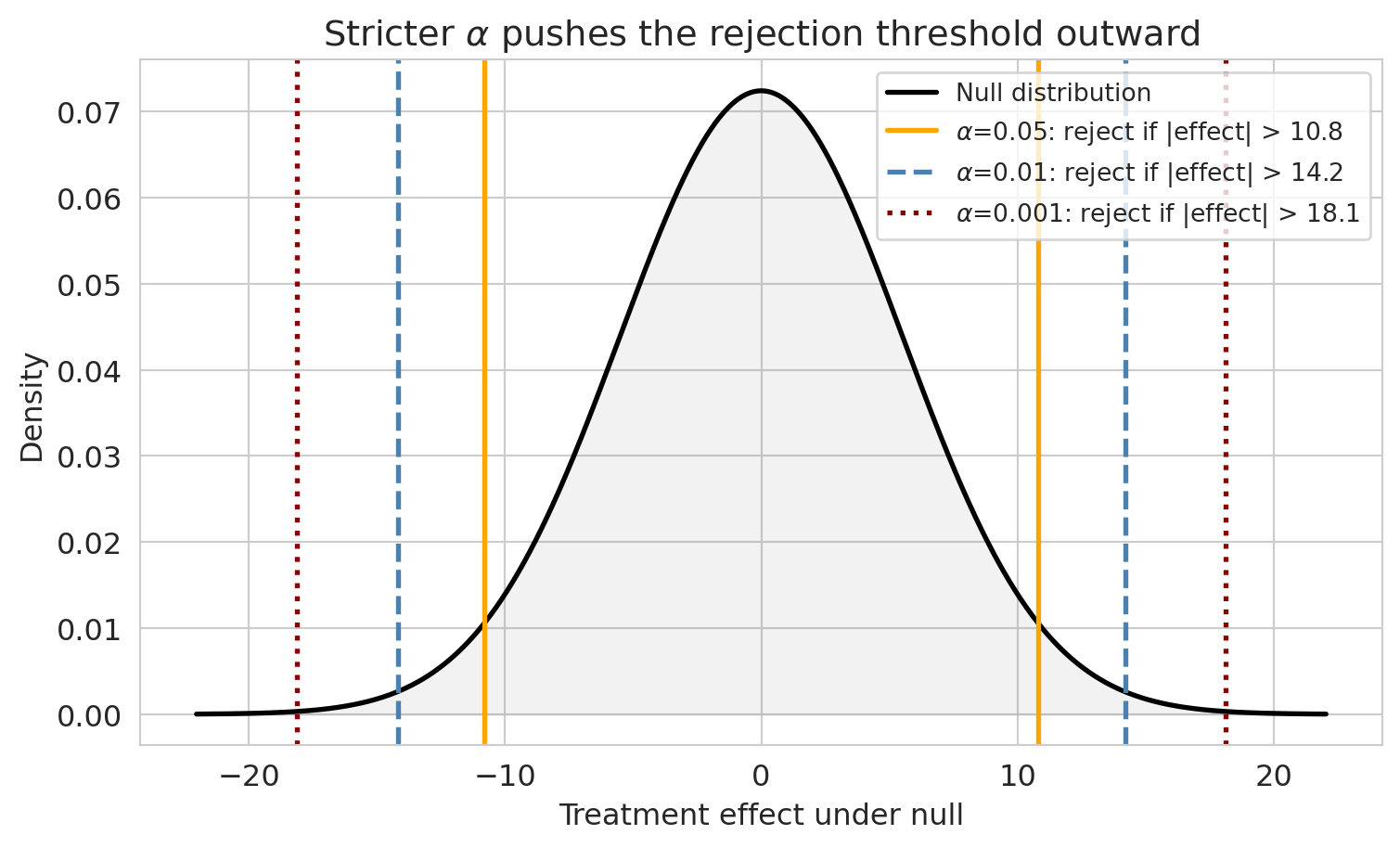
Smaller $\alpha$ means a stricter threshold. That shrinks Type I but inflates Type II, and keeping power up at the stricter threshold requires more patients.
```{python}
null_se = np.sqrt(control.var(ddof=1) / len(control) + treatment.var(ddof=1) / len(treatment))
x = np.linspace(-4*null_se, 4*null_se, 1000)
y = norm.pdf(x, 0, null_se)

fig, ax = plt.subplots(figsize=(9, 5))
ax.plot(x, y, 'k-', lw=2, label='Null distribution')
ax.fill_between(x, y, alpha=0.1, color='gray')

for a_val, color, ls in [(0.05, 'orange', '-'), (0.01, 'steelblue', '--'), (0.001, 'darkred', ':')]:
    cutoff = norm.ppf(1 - a_val/2, 0, null_se)
    ax.axvline(cutoff, color=color, lw=2, ls=ls,
               label=f'$\\alpha$={a_val}: reject if |effect| > {cutoff:.1f}')
    ax.axvline(-cutoff, color=color, lw=2, ls=ls)
ax.set_xlabel('Treatment effect under null'); ax.set_ylabel('Density')
ax.set_title('Stricter $\\alpha$ pushes the rejection threshold outward')
ax.legend(fontsize=10)
plt.show()
```
In practice, the FDA effectively requires two independent positive trials, each at $\alpha = 0.05$. If the trials are truly independent, the joint Type I rate is roughly $0.05^2 = 0.0025$ — far stricter than a single test. (This requirement is the simplest example of a **multiple testing correction**, the topic of [Chapter 11](lec11-multiple-testing.qmd).)
## Confidence intervals and tests: two sides of the same coin
Now that $H_0$, $\alpha$, and "reject" all have crisp definitions, we can close a loop opened in [Chapter 8](lec08-sampling.qmd). There we built a bootstrap 95% CI for the ACTG treatment effect: $[39.6, 61.3]$, excluding zero. Chapter 9 ran the permutation test on the same data and got $p \approx 10^{-4}$ — rejecting $H_0$. The two tools point at the same conclusion, and the agreement is forced by structure.
::: {.callout-important}
## Definition: CI/hypothesis test duality
A 95% CI for a parameter $\theta$ that **excludes** a candidate value $\theta_0$ corresponds exactly to a two-sided test of $H_0: \theta = \theta_0$ that **rejects** at $\alpha = 0.05$. If the interval **includes** $\theta_0$, the test **fails to reject**. The same correspondence holds at any level: a 99% CI pairs with a 1%-level test.
The CI is strictly more informative: it gives you the *range* of plausible parameter values, not just a yes/no verdict on a single one.
:::
The equivalence is **exact** for parametric pairs (normal CI ↔ $z$-test, $t$-CI ↔ $t$-test) and **near-exact** for simulation-based pairs (bootstrap CI ↔ permutation test), with any small gap due to Monte Carlo noise. In practice: **once you have a CI, you have most of what a test would tell you**.
::: {.callout-note collapse="true"}
## Going deeper: verifying the duality on ACTG 175
Recompute Chapter 8's bootstrap CI (resample *within* group, with replacement) and Chapter 9's permutation p-value (shuffle labels *across* groups, without replacement) side by side:
```{python}
np.random.seed(42)
n_boot = 10_000
boot_effects = np.empty(n_boot)
for i in range(n_boot):
    bc = np.random.choice(control, size=len(control), replace=True)
    bt = np.random.choice(treatment, size=len(treatment), replace=True)
    boot_effects[i] = bt.mean() - bc.mean()
ci_lower, ci_upper = np.percentile(boot_effects, [2.5, 97.5])

all_cd4 = np.concatenate([treatment.values, control.values])
n_T = len(treatment)
perm_effects = np.empty(n_boot)
for i in range(n_boot):
    s = np.random.permutation(all_cd4)
    perm_effects[i] = s[:n_T].mean() - s[n_T:].mean()
p_perm = (np.sum(np.abs(perm_effects) >= np.abs(observed_effect)) + 1) / (n_boot + 1)

print(f"Bootstrap 95% CI: [{ci_lower:.1f}, {ci_upper:.1f}]")
print(f"CI excludes 0:    {ci_lower > 0}")
print(f"Permutation p:    {p_perm:.4f}")
print(f"Reject H0 at 5%:  {p_perm < 0.05}")
print(f"Both agree?       {(ci_lower > 0) == (p_perm < 0.05)}")
```
Both agree. In large samples the duality is a restatement.
:::
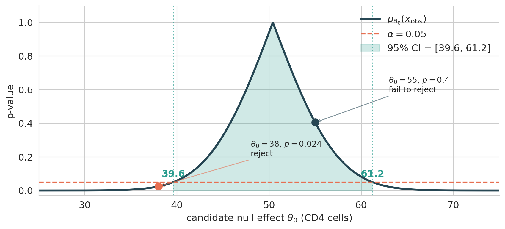
::: {.callout-note collapse="true"}
## Going deeper: the duality is a picture
The cleanest way to see why CI and test agree is to plot the p-value as a function of the candidate null value $\theta_0$, holding the observed data fixed. For a Welch t-test on ACTG 175:
```{python}
#| label: fig-pvalue-curve
#| fig-cap: "p-value curve for ACTG 175. The CI is the super-level set of the curve at height α."
from scipy.stats import t as student_t
import matplotlib.pyplot as plt

xbar = observed_effect
n_T, n_C = len(treatment), len(control)
var_T, var_C = treatment.var(ddof=1), control.var(ddof=1)
se = np.sqrt(var_T/n_T + var_C/n_C)
df_welch = (var_T/n_T + var_C/n_C)**2 / (
    (var_T/n_T)**2 / (n_T - 1) + (var_C/n_C)**2 / (n_C - 1))
alpha = 0.05
t_crit = student_t.ppf(1 - alpha/2, df_welch)
ci_lo, ci_hi = xbar - t_crit*se, xbar + t_crit*se

theta0 = np.linspace(25, 75, 1000)
p_curve = 2 * student_t.sf(np.abs(xbar - theta0)/se, df_welch)

fig, ax = plt.subplots(figsize=(9, 4.2))
ax.plot(theta0, p_curve, color='#264653', lw=2.5, label=r'$p_{\theta_0}(\bar x_{\rm obs})$')
ax.axhline(alpha, color='#e76f51', ls='--', lw=1.6, label=fr'$\alpha = {alpha}$')
ax.fill_between(theta0, 0, p_curve, where=(p_curve > alpha),
                color='#2a9d8f', alpha=0.22,
                label=f'95% CI = [{ci_lo:.1f}, {ci_hi:.1f}]')
ax.axvline(ci_lo, color='#2a9d8f', ls=':', alpha=0.7)
ax.axvline(ci_hi, color='#2a9d8f', ls=':', alpha=0.7)
ax.text(ci_lo, 0.07, f'{ci_lo:.1f}', ha='center', va='bottom',
        color='#2a9d8f', fontweight='bold')
ax.text(ci_hi, 0.07, f'{ci_hi:.1f}', ha='center', va='bottom',
        color='#2a9d8f', fontweight='bold')

for theta_pt, color, verdict in [(55, '#264653', 'fail to reject'),
                                  (38, '#e76f51', 'reject')]:
    p_pt = 2 * student_t.sf(abs(xbar - theta_pt)/se, df_welch)
    ax.plot(theta_pt, p_pt, 'o', color=color, markersize=9, zorder=5)
    ax.annotate(fr'$\theta_0={theta_pt}$, $p={p_pt:.2g}$' '\n' f'{verdict}',
                xy=(theta_pt, p_pt),
                xytext=(theta_pt + (10 if theta_pt < xbar else 8),
                        p_pt + 0.18),
                fontsize=10, ha='left',
                arrowprops=dict(arrowstyle='->', color=color, alpha=0.6))

ax.set_xlabel(r'candidate null effect $\theta_0$ (CD4 cells)')
ax.set_ylabel('p-value')
ax.set_xlim(25, 75); ax.set_ylim(-0.03, 1.10)
ax.legend(loc='upper right', frameon=False)
ax.spines[['top', 'right']].set_visible(False)
plt.tight_layout()
plt.show()
```
The curve peaks at $\theta_0 = \bar x_{\rm obs}$ (where the data are perfectly consistent with the null, so $p = 1$) and decays in both directions. Now read the picture two ways:
- **Confidence interval** = the set of $\theta_0$ where the curve sits *above* $\alpha$. The endpoints (39.6 and 61.2) are exactly where the curve crosses the threshold.
- **Hypothesis test** at any specific $\theta_0$: read the curve at that x-value. Above $\alpha$ → fail to reject; below $\alpha$ → reject.
The CI is precisely the **super-level set** of the p-value curve at height $\alpha$, and the boundary of that level set is exactly where tests flip from "fail to reject" to "reject." (The chapter's null $\theta_0 = 0$ sits off-scale to the left of this plot, with $p \approx 10^{-19}$ — outside the CI, rejected by the test.)
The Welch CI here is $[39.6, 61.2]$; Chapter 8's bootstrap CI was $[39.6, 61.3]$. The 0.1-cell gap at the upper end is bootstrap finite-sample noise — both intervals describe the same underlying parameter, computed two ways.
**A one-line proof.** Suppose for each $\theta_0$ we have a level-$\alpha$ test of $H_0: \theta = \theta_0$ — a decision $\phi_{\theta_0}(X) \in \{0, 1\}$ satisfying $P_{\theta_0}(\phi_{\theta_0}(X) = 1) \le \alpha$. Define the *acceptance set*
$$
C(X) := \{\theta_0 : \phi_{\theta_0}(X) = 0\}.
$$
Then for any true value $\theta$,
$$
P_\theta\!\bigl(\theta \in C(X)\bigr) \;=\; P_\theta\!\bigl(\phi_\theta(X) = 0\bigr) \;=\; 1 - P_\theta\!\bigl(\phi_\theta(X) = 1\bigr) \;\ge\; 1 - \alpha.
$$
Definition of $C$; complements; level guarantee applied at $\theta_0 = \theta$. So $C(X)$ is automatically a $(1-\alpha)$-confidence set; the converse is the same line read right-to-left.
:::
::: {.callout-warning}
## Use hypothesis testing only when you need a binary decision
A clinical trial demands a yes/no verdict on FDA approval. A product launch demands ship/don't-ship. In those settings, hypothesis testing is the right tool. But for *understanding* — "how big is the effect, and how precisely do we know it?" — a confidence interval is almost always more informative.
The most common statistical mistake in industry is using hypothesis testing when estimation would have answered the actual question. If your decision isn't binary, reach for a CI first.
:::
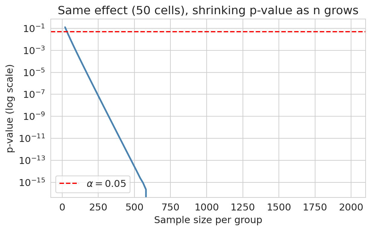
## Statistical significance is not the same as importance
With a large enough $n$, *any* nonzero effect becomes statistically significant. The p-value shrinks as the standard error shrinks; the effect itself does not have to be large.
```{python}
sigma = control.std()
ns = np.arange(20, 2001, 20)
p_vals_vs_n = []
for n in ns:
    se_n = sigma * np.sqrt(2/n)
    t = observed_effect / se_n
    p_vals_vs_n.append(2 * (1 - norm.cdf(abs(t))))

fig, ax = plt.subplots(figsize=(7, 4))
ax.semilogy(ns, p_vals_vs_n, color='steelblue', lw=2)
ax.axhline(0.05, color='red', ls='--', label='$\\alpha=0.05$')
ax.set_xlabel('Sample size per group'); ax.set_ylabel('p-value (log scale)')
ax.set_title(f'Same effect ({observed_effect:.0f} cells), shrinking p-value as n grows')
ax.legend()
plt.show()
```
For a fixed real effect, the p-value collapses as we add data. Eventually *any* nonzero effect becomes significant.
::: {.callout-tip}
## Think about it: the blood pressure drug
A clinical trial with 10,000 participants tests a new blood pressure drug and finds a statistically significant reduction (p = 0.013). The effect: a 2 mmHg decrease in systolic blood pressure. For context, drinking a cup of coffee temporarily raises blood pressure by about 5 mmHg (Mesas et al., *Journal of Hypertension*, 2011). The drug's effect is real — it's not zero — but it's smaller than your morning coffee. Would you recommend this drug to patients, given costs and side effects?
:::
::: {.callout-warning}
## Always report effect sizes alongside p-values
A small p-value tells you the effect is unlikely to be zero. It does **not** tell you the effect is large or important. Always report the effect size (or, equivalently, a CI) so the reader can judge whether the result matters in practice.
:::
A subtler worry follows. When $p < 0.05$ becomes a **target** — when careers and publications depend on clearing that bar — researchers (often unconsciously) run analyses until they find significance. This practice is **p-hacking**, examined in [Chapter 11](lec11-multiple-testing.qmd) — a special case of **Goodhart's law**: a measure that becomes a target stops being a good measure. [Chapter 16](lec16-feedback-loops.qmd) develops the general form — the same pattern that shows up in hospital readmission gaming, emissions cheating, and overfitting.
## Key takeaways
- Hypothesis testing in this chapter is a tool for **designing studies**, not just summarizing data after the fact. The new ideas are error rates, the formula-based t-test, and power analysis.
- The two errors are symmetric: **Type I** (reject $H_0$ when true, rate $\alpha$) and **Type II** (fail to reject $H_0$ when $H_1$ true, rate $\beta$). **Power** $= 1 - \beta$.
- Under $H_0$, p-values from a correctly specified test are **Uniform on $[0,1]$** — that's why $\alpha$ does what it advertises.
- **Welch's t-test** is the formula-based analog of the permutation test: same conclusion in large samples, but solvable for studies you haven't run yet. Use `equal_var=False` by default.
- **Power analysis requires guessing an effect size.** Without that guess there is no calculation. The guess comes from prior studies, the minimum effect worth detecting, or a pilot — and the answer is highly sensitive to the choice.
- **CI/hypothesis test duality**: a 95% CI excluding $\theta_0$ corresponds to a two-sided test of $\theta = \theta_0$ rejecting at $\alpha = 0.05$. The CI is strictly more informative.
- **Use estimation by default; reach for tests when the decision is binary.** Tests are the right tool for ship/don't-ship or approve/reject; for everything else, a CI dominates.
- **Statistical significance is not practical importance.** With enough data, any nonzero effect is "significant." Always report effect sizes.
[Chapter 11](lec11-multiple-testing.qmd) asks: what happens when you run 20 tests at once? [Chapter 12](lec12-regression-inference.qmd) applies hypothesis tests to regression coefficients.
## Study guide
### Key ideas
- **$H_0$ / $H_1$, p-value**: see Chapter 9 for the definitions; this chapter formalizes them and adds error rates.
- **Significance level $\alpha$**: threshold for rejecting $H_0$; equals the Type I error rate.
- **Type I error** (false positive, rate $\alpha$) and **Type II error** (false negative, rate $\beta$). **Power** $= 1 - \beta$.
- **p-values are Uniform(0, 1) under $H_0$**: exact for exact tests (e.g., a fully enumerated permutation test); approximate for large-sample tests like Welch's.
- **Welch's t-test**: the formula-based two-sample test that does not assume equal variances. The standard default.
- "Fail to reject" is not the same as "accept."
- **CI/test duality**: a $(1-\alpha)$-level CI for $\theta$ excluding $\theta_0$ ↔ two-sided test of $\theta = \theta_0$ rejecting at level $\alpha$. The CI is strictly more informative.
- **Power analysis**: you must commit to an effect size to compute required $n$. The 80% target is convention.
- Statistical significance does not imply practical importance; always report effect sizes.
### Computational tools
- `stats.ttest_ind(a, b, equal_var=False)` — Welch's t-test for two independent samples
- `TTestIndPower().solve_power(effect_size, power, alpha)` — required sample size given Cohen's $d$, target power, and $\alpha$
- `TTestIndPower().solve_power(effect_size, nobs1, alpha)` — power given sample size
### For the quiz
- State $H_0$ and $H_1$ for a given scenario and identify the appropriate test.
- Distinguish Type I and Type II errors and explain how $\alpha$ controls the tradeoff.
- Read a power curve and explain what changes power.
- Given a target power and an assumed effect size, identify the required sample size from a power tool — and explain why the assumed effect size is the most consequential input.
- Use CI/test duality to convert between a CI and a two-sided test decision.
- Explain why a large sample can make a tiny, meaningless effect "significant."