Working with AI

  Download notebook (.ipynb)

You can give a dataset to an AI tool today — a chat interface with a code interpreter, a notebook agent, an AutoML pipeline — and get a fitted model and a written analysis back in seconds. When should you trust the result? What is the human still responsible for?

The chapter’s throughline: AI tools have automated the mechanical step, not the judgment step. We cover three classes of 2026 automation — AutoML for model selection, tabular foundation models that skip per-dataset training, and LLM agents that write analysis pipelines. For each, we examine what published benchmarks say it does well, where it still fails, and what the human contributes that the tool cannot. The chapter closes with a checklist for evaluating any analysis — a colleague’s, a vendor’s, or an AI’s — delivering the promise from Chapter 1.

import numpy as np
import pandas as pd
import matplotlib.pyplot as plt
import seaborn as sns
from scipy import stats
from sklearn.linear_model import LinearRegression
from sklearn.ensemble import RandomForestRegressor, GradientBoostingRegressor
from sklearn.model_selection import cross_val_score, KFold
from sklearn.preprocessing import StandardScaler
from sklearn.pipeline import Pipeline
import warnings
warnings.filterwarnings('ignore')
sns.set_style('whitegrid')
plt.rcParams['figure.figsize'] = (7, 4.5)
plt.rcParams['font.size'] = 12

DATA_DIR = 'data'

Gradient boosting: the model AutoML searches over

Random forests and gradient boosting from Chapter 13 are the first models any AutoML system will try on tabular data. The forest mechanism — bootstrap sampling, feature subsets, average independently-grown trees — you already know. We cover gradient boosting here because it is the algorithm behind XGBoost, LightGBM, and CatBoost, the libraries that win most tabular competitions.

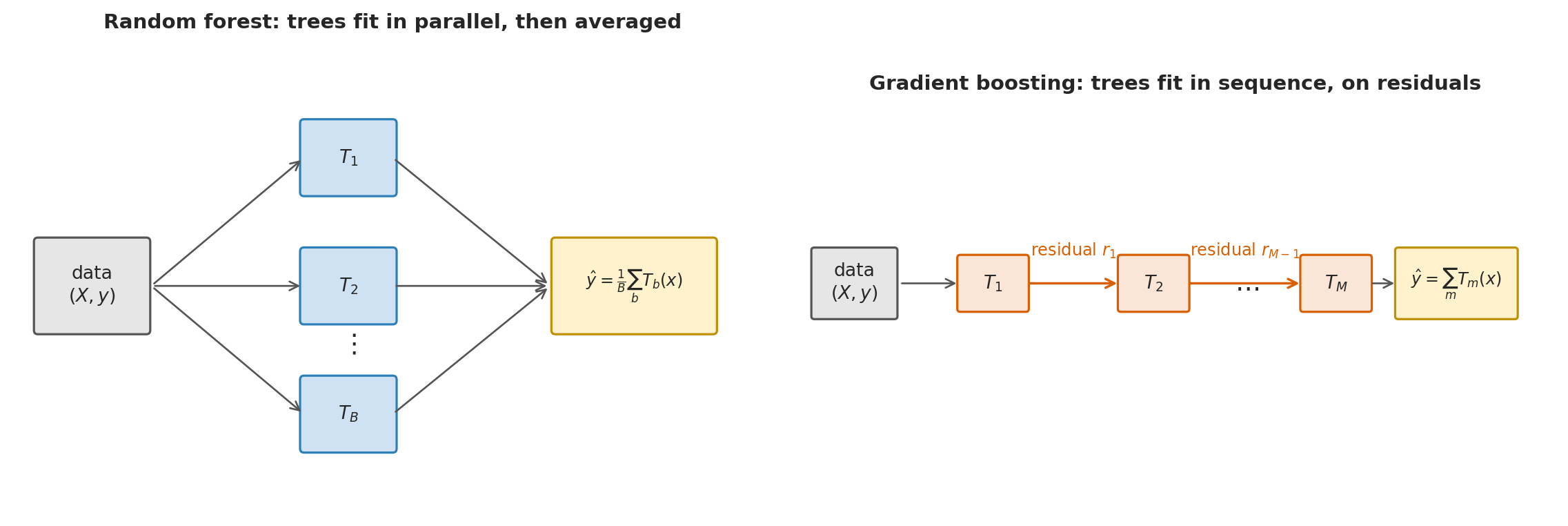
Where a forest averages many trees grown in parallel, gradient boosting grows them sequentially: each new tree is trained on the errors of the previous trees.

Each new tree fits the residuals of the ensemble so far, so the ensemble’s prediction error shrinks with every tree added. For squared-error loss the residual is just \(y - \hat y\); for classification or other losses the same procedure applies but “residual” means the gradient of that loss.

Random forest fits trees in parallel and averages their predictions; gradient boosting fits trees in sequence, with each tree trained on the residuals of the previous ensemble.

NoteGoing deeper: gradient boosting as gradient descent in function space

Let \(F(x)\) denote the current ensemble’s prediction. The pseudo-residual at training point \(x_i\) is the negative partial derivative of the loss with respect to \(F(x_i)\): \[r_i = -\frac{\partial L_i}{\partial F(x_i)}.\] Each gradient-boosting step fits a regression tree to predict the pseudo-residuals from \(x\), and adds (a scaled copy of) that tree to the ensemble. Where gradient descent (Chapter 7) updates parameters against a loss gradient, gradient boosting updates a function.

Squared-error loss. \(L_i = \tfrac{1}{2}(y_i - F(x_i))^2\), so \(r_i = y_i - F(x_i)\) — the ordinary prediction error. Each tree fits the previous ensemble’s mistakes.

Logistic loss (\(y_i \in \{0,1\}\), \(F(x_i)\) the logit, \(p_i = \sigma(F(x_i))\)). \(L_i = -y_i \log p_i - (1-y_i)\log(1-p_i)\), and the chain rule through \(\sigma\) gives \(r_i = y_i - p_i\) — the gap between observed label and predicted probability.

# Predict Airbnb listing price from numeric + one-hot categorical features
listings = pd.read_csv(f'{DATA_DIR}/airbnb/listings.csv', low_memory=False)
listings['price'] = pd.to_numeric(
    listings['price'].astype(str).str.replace(r'[$,]', '', regex=True),
    errors='coerce')
listings = listings[listings['price'].between(10, 500)]

num_cols = ['bedrooms', 'bathrooms', 'accommodates', 'number_of_reviews',
            'latitude', 'longitude']
cat_cols = ['room_type', 'neighbourhood_group_cleansed']
listings_clean = listings[num_cols + cat_cols + ['price']].dropna()

X = pd.concat([
    listings_clean[num_cols],
    pd.get_dummies(listings_clean[cat_cols], drop_first=True)
], axis=1)
y = listings_clean['price']

forest = RandomForestRegressor(n_estimators=200, random_state=42)
forest_cv = cross_val_score(forest, X, y, cv=5, scoring='r2')

gboost = GradientBoostingRegressor(n_estimators=200, max_depth=4, random_state=42)
gboost_cv = cross_val_score(gboost, X, y, cv=5, scoring='r2')

print(f"Random Forest:     CV R-sq = {forest_cv.mean():.3f}")
print(f"Gradient Boosting: CV R-sq = {gboost_cv.mean():.3f}")

Random Forest:     CV R-sq = 0.642
Gradient Boosting: CV R-sq = 0.668

On this Airbnb pricing task gradient boosting outperforms the random forest. Sequential error-correction picks up the feature interactions and price discontinuities that the forest’s bagging averages over. Production gradient-boosting libraries (XGBoost, LightGBM, CatBoost) add learning-rate shrinkage, second-order gradients, regularization, and refined splitting rules that scikit-learn’s reference implementation lacks; with those, the gap typically widens. A 2022 benchmark across 45 datasets settled a long-running debate: tree-based models still outperform deep neural networks on typical tabular data, because tabular features are heterogeneous and tabular targets are non-smooth in ways that the rotational invariance of neural networks does not handle well.¹ Trees and forests are the default tabular model family for AutoML.

The AutoML loop

ImportantDefinition: AutoML

AutoML (automated machine learning) is software that, given a dataset and a target, searches a space of model families and hyperparameters and returns a fitted pipeline. Open-source examples include AutoGluon, FLAML, auto-sklearn, H2O AutoML, and TPOT; cloud examples include Google Vertex AI, AWS SageMaker Autopilot, and Azure AutoML.

CASH: combined algorithm selection and hyperparameter optimization

In Chapter 13 you swept candidate tree depths, scored each by 5-fold cross-validation, and picked the depth with the best score — the same recipe Chapter 6 used for polynomial degree and lasso \(\alpha\). AutoML scales that recipe up: instead of sweeping one hyperparameter inside one model family, it searches over algorithm choices and all their hyperparameters at once. The task the field calls CASH — Combined Algorithm Selection and Hyperparameter optimization — is exactly this loop, automated and searched systematically. Auto-WEKA introduced the name in 2013 by folding “which algorithm” into a single top-level categorical hyperparameter, turning algorithm choice and hyperparameter tuning into one optimization problem.²

A minimal AutoML in a few sklearn lines: try three model families — linear regression, a random forest, and gradient boosting — with cross-validation, and select the best. The Pipeline wrap on the linear model — Pipeline([('scaler', StandardScaler()), ('model', LinearRegression())]) — fits StandardScaler only on each training fold, so the scaler never sees the held-out fold’s mean and standard deviation. This is the same loop AutoML automates at larger scale.

# Poor man's AutoML on the Airbnb data: try 3 models, pick the best by 5-fold CV.
# Pipeline keeps the scaler from leaking test-fold info into training.
kf = KFold(n_splits=5, shuffle=True, random_state=42)

models = {
    'Linear Regression': Pipeline([('scaler', StandardScaler()), ('model', LinearRegression())]),
    'Random Forest\n(200 trees)': RandomForestRegressor(n_estimators=200, random_state=42),
    'Gradient Boosting\n(200 trees)': GradientBoostingRegressor(n_estimators=200, max_depth=4, random_state=42),
}

cv_results = {}
print(f"{'Model':<35} {'Mean R-sq':>10} {'Std':>8} {'Mean MAE':>10}")
print("=" * 68)
best_score = -np.inf
best_name = None

for name, model in models.items():
    r2_scores = cross_val_score(model, X, y, cv=kf, scoring='r2')
    mae_scores = -cross_val_score(model, X, y, cv=kf, scoring='neg_mean_absolute_error')
    cv_results[name] = r2_scores
    display_name = name.replace('\n', ' ')
    print(f"{display_name:<35} {r2_scores.mean():>10.3f} {r2_scores.std():>8.3f} {mae_scores.mean():>10.1f}")
    if r2_scores.mean() > best_score:
        best_score = r2_scores.mean()
        best_name = display_name

print(f"\nWinner: {best_name} (R-sq = {best_score:.3f})")

Model                                Mean R-sq      Std   Mean MAE
====================================================================
Linear Regression                        0.569    0.009       38.3
Random Forest (200 trees)                0.641    0.008       33.1
Gradient Boosting (200 trees)            0.668    0.007       32.0

Winner: Gradient Boosting (200 trees) (R-sq = 0.668)

# Visualize the CV results
fig, ax = plt.subplots(figsize=(8, 5))
bp = ax.boxplot([scores for scores in cv_results.values()],
                tick_labels=list(cv_results.keys()),
                patch_artist=True)
colors = ['#4C72B0', '#F0A30A', '#C44E52']
for patch, color in zip(bp['boxes'], colors):
    patch.set_facecolor(color)
    patch.set_alpha(0.7)
ax.set_ylabel('R-squared (5-fold CV)')
ax.set_title('Mini AutoML shootout: predicting Airbnb listing price')
ax.grid(axis='y', alpha=0.3)
plt.tight_layout()
plt.show()

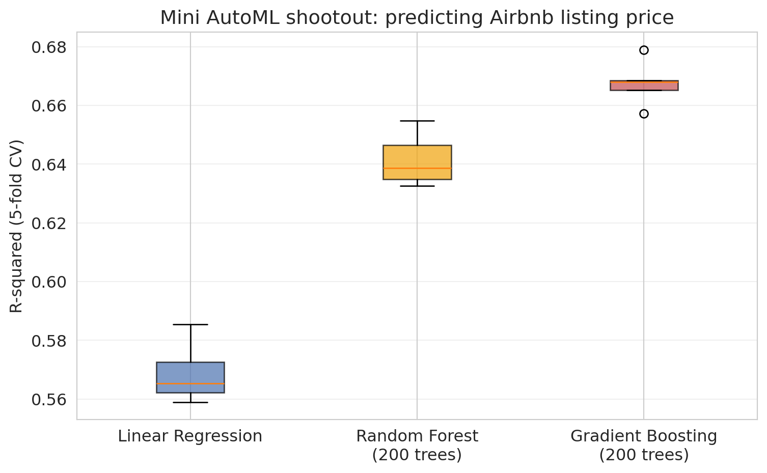
Notice how much the per-fold scores overlap. The difference in mean CV R-sq between configurations is often small compared with the spread across folds, so on a different sample of folds the ordering could easily reverse. Real AutoML systems handle this with the same idea a random forest already uses: average the predictions from several configurations — a numeric average for regression, a majority vote for classification — instead of picking just one. That ensemble step turns out to be the lever the next subsection cares about.

Beyond grid search, the modern toolkit is random search,³ Bayesian optimization with model-based surrogates, and bandit-style early stopping that drops the lowest-performing configurations on cheap evaluations before the expensive ones — Hyperband is the standard reference.⁴

TipThink about it

Before we continue — what did AutoML not do here? Which decisions did we make before any model was fit?

AutoGluon wins by ensembling, not by better search

The 2024 benchmark of record on tabular AutoML — nine frameworks, 71 classification tasks and 33 regression tasks — found a clear leader.⁵ AutoGluon is the strongest open-source AutoML system on tabular data — and the reason is not a more sophisticated search algorithm. The gains come from ensembling and multi-layer stacking of many models AutoGluon has already fit. Stacking trains a small meta-learner whose input features are the predictions of the base models; the meta-learner learns which base model to trust under which conditions, and combines their predictions so individual errors cancel. Both moves confirm a 2004 result on ensemble selection from libraries of models that predates the entire AutoML era.⁶

The 2026 frontier is no longer about better search algorithms. The improvements come from (a) ensembling models you have already fit and (b) reusing structure across datasets — the subject of the next section.

Tabular foundation models

Foundation models — single large pretrained networks adapted to many downstream tasks — became the norm in language (GPT, Claude, Gemini) and vision (CLIP, SAM) over the last several years. Tabular data is catching up. The leading example is TabPFN.

ImportantDefinition: TabPFN

TabPFN (Tabular Prior-data Fitted Network) is a transformer pretrained once, offline, on millions of synthetic tabular datasets. At deployment it does no training and no hyperparameter tuning: paste the entire training table into the model’s context window, append the test rows, read predictions off in one forward pass. Current v2 caps out around 10,000 rows and 500 features.

This is in-context learning — the same mechanism that lets large language models produce a sensible answer from a few examples in a prompt, applied to tables. The result was first published at ICLR 2023⁷ and substantially expanded in Nature in January 2025:⁸ a single pretrained model with no per-dataset fitting outperforms tuned XGBoost and CatBoost on small tabular problems. The version-2 release adds regression alongside classification, and TabICL (ICML 2025) extends the same approach to datasets with hundreds of thousands of rows.⁹

For twelve years the unstated assumption in AutoML was search for the right model on each new dataset. A pretrained tabular foundation model breaks that assumption: the same model serves every dataset, and what changes is the example table placed in the context window. TabPFN v2 needs a GPU for inference, so it does not replace AutoML on every problem. It currently leads on small datasets, where pretraining across datasets helps most.

NoteTabPFN on the Airbnb data, head-to-head

On a 10,000-row subsample of the Airbnb pricing task above (TabPFN v2’s row cap), TabPFN with no hyperparameter search at all beats the tuned gradient booster on the same subsample:

Model	5-fold CV R²
Random forest (n_estimators=200)	0.636
Gradient boosting (n_estimators=200, max_depth=4)	0.652
TabPFN v2 (defaults)	0.668

The chapter does not run TabPFN at render time — it adds a GPU-leaning dependency outside the book’s CI environment. Reproduce the numbers above with scripts/lec17-tabpfn-benchmark.py.

LLM agents writing data-analysis pipelines

Alongside AutoML and foundation models, a third class of tools is large language models that write, execute, and revise analysis code.

ImportantDefinition: AI agent (for data analysis)

A data-analysis agent is a control loop around a language model: the model proposes code; an interpreter runs it; the model reads the output (numbers or tracebacks); the model revises and iterates. The agent is the loop, not the language model alone. Modern tools differ in how the loop is structured (single planner, multi-agent debate, tree search over code), but they all execute and read back.

Two examples carry useful through-lines for this chapter:

• CAAFE — the LLM reads a dataset description and proposes new features as code plus an explanation.¹⁰ Same group as TabPFN; in their stack an LLM does the feature engineering and a pretrained transformer does the modelling.
• AIDE — runs machine-learning engineering as a tree search over candidate code.¹¹ Conceptually CASH, but the search space is programs rather than (algorithm, hyperparameters) tuples.

Other 2024–2025 systems take similar shapes — graph-of-tool-calls planners (Data Interpreter / MetaGPT) and multi-agent reader-planner-developer loops (AutoKaggle) — converging on the same overall pattern.¹²

How well do they actually do? OpenAI’s MLE-bench measures this directly: 75 real Kaggle competitions, scored against the published human leaderboards.¹³ In the original paper the best setup — o1-preview with the AIDE scaffold — reached at least a bronze medal in 16.9% of competitions. The public leaderboard has since climbed: as of early 2026 the top entry, R&D-Agent (o3 + GPT-4.1), reports a roughly 30% medal rate, with new submissions paused 2026-04-24 pending a fairness review. Even the better number means today’s best agents fail to clear the lowest human medal tier in about two of every three competitions.

The trend across all three classes — AutoML, foundation models, agents — is convergence. AIDE’s tree search over code is CASH over programs. CAAFE is an LLM feeding features into a downstream tabular model. Agents increasingly call AutoGluon, XGBoost, or TabPFN as tools rather than reimplementing them.

Honest capability boundaries

Where do these tools still fail? The 2026 benchmark picture is fairly consistent.

Reliable on the mechanical step, unreliable on the judgment-laden workflow. DABStep is currently the closest benchmark to “an analyst doing real work” — 450+ multi-step data-analysis tasks drawn from a financial-analytics platform, partitioned into Easy and Hard tiers by the benchmark authors.¹⁴ On the Easy tier, a frontier model scores about 76%. On the Hard tier — same model, same dataset, but the task requires reasoning across multiple documents and code steps — it scores about 15%. That 76/15 gap is the failure profile. The arithmetic step is mostly solved; the judgment that connects one step to the next is not.

Other benchmarks show the same pattern: about 25% on open-ended hypothesis discovery (DiscoveryBench), about 30% on real-world data-wrangling code generation (DA-Code), and on BLADE — which scores analytical decisions against the range of choices expert data scientists would defend — about 27% agreement on data transformations and 13% on conceptual-variable choices.¹⁵ The tools converge on a narrow set of analytic choices, not the breadth a careful analyst would weigh.

One-shot versus tool-using agent

It matters whether the AI is just writing code or also executing it. A model that emits code without running it can return a plausible-looking wrong number — for example, prose claiming p = 0.03 for a test the code never actually ran. An agent that executes the code and reads the output cannot fabricate the printed number; the traceback or the printed value forces a correction.

So execution removes the crash class of errors — syntax bugs, wrong column names, shape mismatches, fabricated numbers in prose. Execution does not remove the judgment class — wrong test for the data, train–test leakage, mis-framed question, unchecked assumption. Those run cleanly and return a wrong-but-plausible answer. The distinction:

Execution lets you trust the arithmetic. It does not let you trust the analysis design, the assumption checking, or the causal interpretation.

How well-calibrated is an AI tool’s confidence?

The literature here is more nuanced than the popular claim “LLMs are confidently wrong” suggests. Base language models — before reinforcement-learning-from-human-feedback (RLHF) post-training — are well-calibrated; GPT-4’s pretraining checkpoint scored close to perfect calibration on multiple-choice benchmarks.¹⁶ The post-training that turns a base model into a chat assistant reduces that calibration.

The loss is largely recoverable with simple prompting. On QA benchmarks like TriviaQA, SciQ, and TruthfulQA, asking the model for several candidate answers before its confidence score cuts its miscalibration — the gap between stated confidence and empirical accuracy — by about 50% relative.¹⁷ Anthropic’s own work shows large language models can usefully estimate the probability that their own answers are correct.¹⁸

The accurate statement: an unprompted “I am confident” from a chat model carries little statistical meaning, but the underlying calibration is recoverable. When it matters, get assurance from re-running, cross-checking, and your own assumption checks — not from the tool’s stated confidence.

What is documented, what is not

Two failure modes are documented well enough to teach as defaults:

• Skipping assumption checks unless explicitly asked. A 2023 validation study found ChatGPT routinely omitted the assumptions of the tests it recommended (normality, equal variance, independence) and gave divergent answers about which test to use.¹⁹ A 2025 healthcare-research validation reports overall inferential accuracy of 32.5% on bare prompts, 81.3% on prompts that named the test, and 92.5% on prompts that also listed which assumptions to check²⁰ — the same tool, made reliable by the analyst’s specification. The pattern is omission unless asked.
• Output quality is highly sensitive to prompt specificity. On identical analytical tasks, accuracy in the Ruta study nearly tripled as the prompt became more specific. The tool does the work you specify and skips the work you do not.

Two more failure modes are weakly documented enough that we should not assert them in stronger language than the evidence supports:

• “Confuses correlation with causation.” Language models are documented to struggle on formal causal-reasoning text benchmarks (CLadder; Causal Parrots),²¹ but no published study measures how often a data-analysis agent specifically reports a regression coefficient as a causal effect. Treat correlation-vs-causation as a known limitation of statistical reasoning generally — humans do this too — not as a measured AI failure rate.
• “Agents p-hack on their own.” The documented phenomenon is researchers exploiting LLM configuration choices to fish for the result they want — “prompt-hacking” or “LLM-hacking.”²² That is a human-misuse risk amplified by the tool, not autonomous agent behavior.

The short version: the tool does the work you specify and skips the work you do not. Your job moves from running the analysis to specifying it, supplying the checklist, and auditing the result. The failures that survive code execution are precisely the failures of judgment — exactly the part of statistics this course has trained you to check.

The failure-profile axes

Four axes of variation organize the picture:

Axis of variation	Reliable when…	Unreliable when…	Empirical anchor
Task complexity	single-step, well-specified	multi-step, open-ended	DABStep Easy ~76% vs Hard ~15%
Prompt specificity	the analyst names the test + lists assumptions	the prompt is bare	Ruta 2025: 32.5% → 81.3% → 92.5%
Execution	the agent runs the code and reads the output	one-shot text only	Execution removes fabricated-in-prose numbers; judgment-class errors persist
Model variant (RLHF stage)	base model, or chat model with a calibration prompt	unprompted RLHF-tuned chat	GPT-4 base calibrated; verbalized chat overconfident unless asked

Three of these axes — task complexity, prompt specificity, execution — you can control by how you use the tool. (Model variant is fixed by which system you call.) Prompt decomposition, later in this chapter, works on exactly these axes: it breaks a hard, open task into a sequence of small specified ones, shifting prompt specificity toward the right and task complexity toward the easy end. Arithmetic-class errors get removed as you move along these axes; judgment-class errors — wrong test, leakage, mis-framed question, unchecked assumption — remain.

Worked examples: where judgment makes the difference

Two analyses make this concrete. The first is about who the data omits; the second is about confounding inside the data we have. Both are mistakes a hurried analyst — human or AI — will make without a deliberate check.

Example 1: silent data loss on the College Scorecard

Consider a different dataset — the College Scorecard, one row per US institution with information on enrollment, financial aid, and graduate earnings. A standard analysis predicts ten-year graduate earnings from a handful of school characteristics; the simple recipe is “drop the rows with missing values, then fit a model.” Look at what that drops.

# Load College Scorecard and apply the standard complete-case filter
scorecard = pd.read_csv(f'{DATA_DIR}/college-scorecard/scorecard.csv')

scorecard_features = ['SAT_AVG', 'UGDS', 'PCTPELL', 'PCTFLOAN', 'RET_FT4',
                      'C150_4_POOLED_SUPP', 'CONTROL']
scorecard_target = 'MD_EARN_WNE_P10'

for col in scorecard_features + [scorecard_target]:
    scorecard[col] = pd.to_numeric(scorecard[col], errors='coerce')

scorecard_complete = scorecard[scorecard_features + [scorecard_target]].dropna()

print("Institutions with complete data vs. all institutions:")
print(f"  All institutions:    {len(scorecard):,}")
print(f"  With SAT_AVG:        {scorecard['SAT_AVG'].notna().sum():,}")
print(f"  With earnings data:  {scorecard[scorecard_target].notna().sum():,}")
print(f"  Complete cases:      {len(scorecard_complete):,}")

Institutions with complete data vs. all institutions:
  All institutions:    7,703
  With SAT_AVG:        1,304
  With earnings data:  5,693
  Complete cases:      1,236

# Which kinds of schools survive the filter?
scorecard_analysis = scorecard.copy()
scorecard_analysis['has_data'] = scorecard.index.isin(scorecard_complete.index)
control_labels = {1: 'Public', 2: 'Private nonprofit', 3: 'Private for-profit'}
scorecard_analysis['control_label'] = pd.to_numeric(scorecard_analysis['CONTROL'], errors='coerce').map(control_labels)

retention_data = []
print("Representation by institution type:")
for label in ['Public', 'Private nonprofit', 'Private for-profit']:
    total = (scorecard_analysis['control_label'] == label).sum()
    kept = ((scorecard_analysis['control_label'] == label) & scorecard_analysis['has_data']).sum()
    if total > 0:
        pct = kept / total
        print(f"  {label:<25s} {kept:>5d} / {total:>5d} ({pct:.0%} kept)")
        retention_data.append({'type': label, 'kept': kept, 'total': total, 'pct': pct})

Representation by institution type:
  Public                      483 /  2044 (24% kept)
  Private nonprofit           748 /  1956 (38% kept)
  Private for-profit            5 /  3703 (0% kept)

# Visualize the selection bias — sort so the headline 0% reads at the top of the chart
retention_df = pd.DataFrame(retention_data).sort_values('pct', ascending=False)
color_map = {'Public': '#4C72B0', 'Private nonprofit': '#F0A30A', 'Private for-profit': '#C44E52'}
fig, ax = plt.subplots(figsize=(8, 4))
bars = ax.barh(retention_df['type'], retention_df['pct'], color=[color_map[t] for t in retention_df['type']])
ax.set_xlabel('Fraction retained in analysis')
ax.set_title('Which schools survive the missing-data filter?')
ax.set_xlim(0, 1)
for bar, (_, row) in zip(bars, retention_df.iterrows()):
    ax.text(bar.get_width() + 0.02, bar.get_y() + bar.get_height()/2,
            f"{row['pct']:.0%}", va='center')
plt.tight_layout()
plt.show()

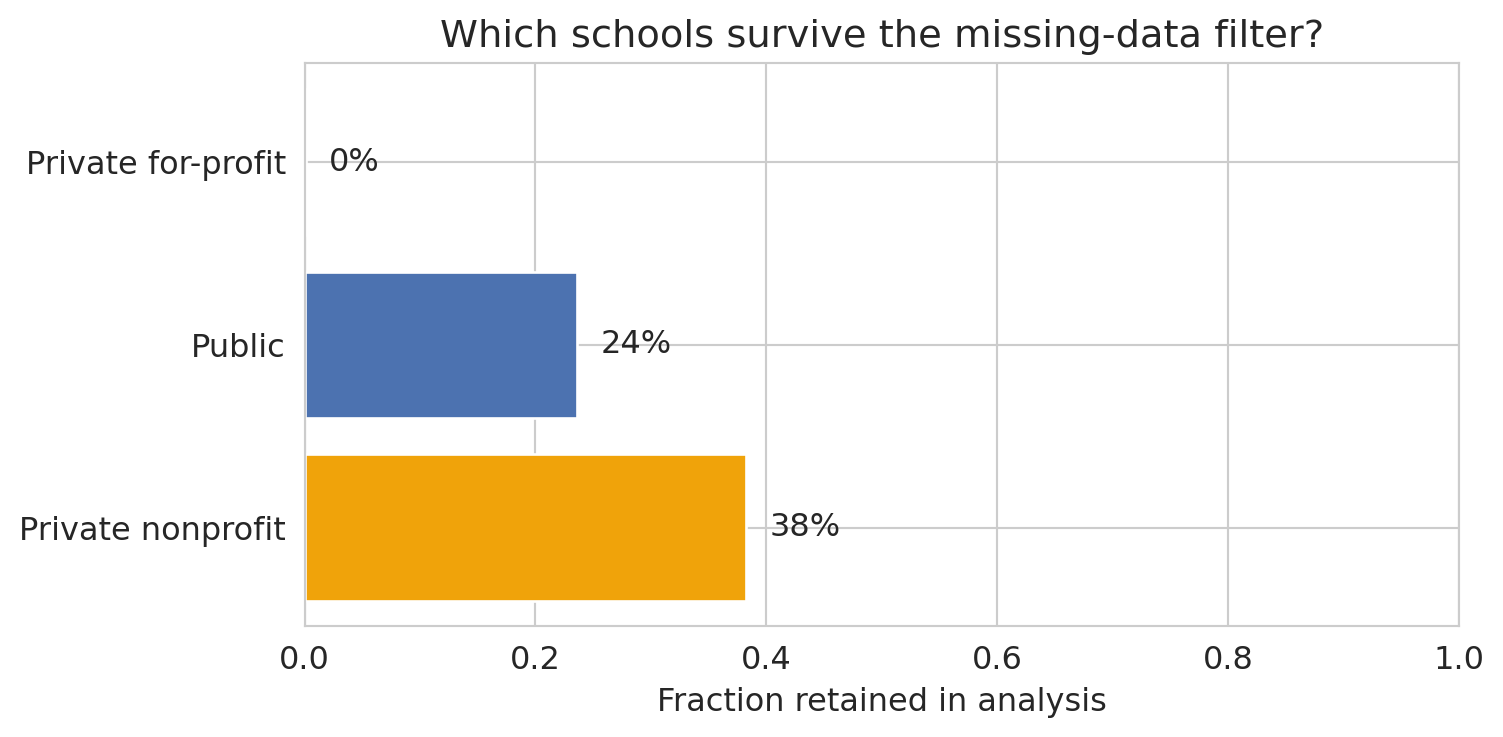
The exclusion pattern is selection bias from Chapter 3 — the MNAR (missing not at random) case. Requiring SAT scores excludes community colleges, trade schools, and most for-profit institutions — precisely the schools where the relationship between institutional characteristics and earnings is likely to be different from the schools we kept. AutoML, foundation models, and LLM agents will all fit a model on the rows that remain and report a respectable cross-validated R². None of them will tell you which schools the analysis no longer applies to. That is a judgment call upstream of any fit.

Example 2: Simpson’s paradox in NBA rest days

A practiced analyst — or a chat assistant given a vague prompt like “do NBA players score more when rested?” — would start with the simplest comparison: select the player-game rows where rest was at least 3 days, select the rows where rest was at most 1, t-test the means.

# Load NBA data
nba = pd.read_csv(f'{DATA_DIR}/nba/nba_load_management.csv')
nba['GAME_DATE'] = pd.to_datetime(nba['GAME_DATE'])
print(f"NBA dataset: {len(nba):,} player-games")
print(f"Seasons: {nba['SEASON'].unique()}")

NBA dataset: 78,335 player-games
Seasons: <StringArray>
['2021-22', '2022-23', '2023-24']
Length: 3, dtype: str

# The tempting first-pass analysis: compare rested vs not-rested across all players
rested = nba[nba['REST_DAYS'] >= 3]['PTS']
not_rested = nba[nba['REST_DAYS'] <= 1]['PTS']

t_stat, p_value = stats.ttest_ind(rested, not_rested)

print("'Do players score more when rested?'")
print(f"  Rested (3+ days):      {rested.mean():.1f} PPG (n={len(rested):,})")
print(f"  Not rested (0-1 days): {not_rested.mean():.1f} PPG (n={len(not_rested):,})")
print(f"  t-statistic: {t_stat:.2f}")
print(f"  p-value: {p_value:.2e}")

'Do players score more when rested?'
  Rested (3+ days):      9.3 PPG (n=23,653)
  Not rested (0-1 days): 11.3 PPG (n=11,288)
  t-statistic: -20.50
  p-value: 7.78e-93

Rested players score fewer points than not-rested players, and the difference is overwhelmingly statistically significant. That is backwards from what you would expect.

TipThink about it

Why might this be backwards? Pause for 30 seconds before reading on. What features of the player pool could drive a difference like this without rest itself being the cause?

The reversal is Simpson’s paradox from Chapter 11. The aggregate comparison is backwards because rest days are confounded with player quality:

• Bench players (low scorers) have more rest days — they do not play every game.
• Stars (high scorers) play on back-to-backs — coaches need them on the floor.

The naive test also calls ttest_ind as if each player-game were independent, when in fact the same players appear many times across games. The independence assumption is violated.

The careful version controls for player identity. The within-player analysis switches from raw PTS to GAME_SCORE, a composite metric that accounts for rebounds, assists, turnovers, and efficiency.

# Within-player comparison (the right shape of analysis, from Lecture 11)
player_effects = []
players_tested = 0
significant_naive = 0

for player in nba['PLAYER_NAME'].unique():
    pdata = nba[nba['PLAYER_NAME'] == player]
    rested_p = pdata[pdata['REST_DAYS'] >= 3]['GAME_SCORE']
    tired_p = pdata[pdata['REST_DAYS'] <= 1]['GAME_SCORE']

    if len(rested_p) >= 10 and len(tired_p) >= 10:
        t, p = stats.ttest_ind(rested_p, tired_p)
        players_tested += 1
        if p < 0.05:
            significant_naive += 1
        player_effects.append({
            'player': player,
            'diff': rested_p.mean() - tired_p.mean(),
            'p_value': p
        })

# Summarize the within-player results
effects_df = pd.DataFrame(player_effects)

print(f"Within-player analysis:")
print(f"  Players tested: {players_tested}")
print(f"  'Significant' at p<0.05: {significant_naive} ({significant_naive/players_tested:.1%})")
print(f"  Expected by chance (5%): {players_tested * 0.05:.0f}")
print()
print(f"  Mean effect (rested - tired): {effects_df['diff'].mean():+.2f} game score points")
print(f"  Median effect:                {effects_df['diff'].median():+.2f}")

Within-player analysis:
  Players tested: 431
  'Significant' at p<0.05: 37 (8.6%)
  Expected by chance (5%): 22

  Mean effect (rested - tired): -0.59 game score points
  Median effect:                -0.63

# Visualize the distribution of per-player effects
fig, ax = plt.subplots(figsize=(8, 4.5))
ax.hist(effects_df['diff'], bins=25, color='steelblue', edgecolor='white', alpha=0.85)
ax.axvline(x=0, color='black', linestyle='-', linewidth=1, label='No effect (0)')
ax.axvline(x=effects_df['diff'].mean(), color='#d62728', linestyle='--', linewidth=2,
           label=f"Within-player mean = {effects_df['diff'].mean():+.2f}")
ax.set_xlabel('Per-player effect: mean game score rested − mean game score tired')
ax.set_ylabel('Number of players')
ax.set_title("Per-player rested-minus-tired effect distribution")
ax.legend()
plt.tight_layout()
plt.show()

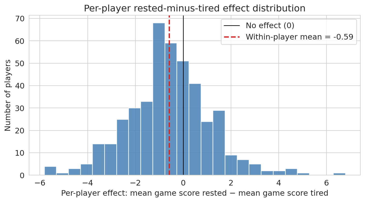
Most players sit near zero. The mean is shifted by under one game-score point against rest — small relative to typical game-to-game variability. Once player identity is controlled for, the large aggregate difference disappears: it came mostly from confounding between rest and player quality, not from a real effect of rest on performance. The per-player test still flags a single-digit-percent subset as “significant” at the 5% level — modestly more than chance alone would predict, but consistent with most of those being false positives from multiple testing across hundreds of players (Chapter 11).

The arithmetic in the first pass was correct. The judgment was wrong. Knowing this required the chapters that came before: Simpson’s paradox and within-subject comparisons (Chapter 11), multiple-testing inflation (Chapter 11), practical-significance reasoning (Chapter 12). An AI tool will produce the first pass in seconds. The audit is where statistical training matters.

What remains irreducibly human

AI tools are improving rapidly. Some parts of the work remain human.

Asking the right question. “What predicts earnings?” is a different question from “What causes higher earnings?” or “Which schools provide the most value-added?” The data alone cannot tell you which question to ask.

Knowing the domain. Why are for-profit schools missing SAT data? Why do bench players have more rest days? Why does AQI spike in August? Domain knowledge is the difference between a plausible-looking wrong answer and a correct one.

Questioning assumptions. Every statistical method makes assumptions. An automation will fit cleanly and report a number even when those assumptions are violated. You now know to ask: Is this data representative? Is the relationship causal? Are the residuals well-behaved? Are we testing too many hypotheses?

Understanding stakes and consequences. A wrong prediction about air quality could mean people go outside during a hazardous event. A wrong conclusion about school quality could redirect billions in funding. The statistical method is the same; the consequences are not.

Communicating uncertainty honestly. Default AI outputs project confidence; good statisticians communicate uncertainty. “The model suggests X, but the confidence interval is wide and the data is missing for the most vulnerable populations” is more honest — and more useful — than “X.”

NoteTukey on asking the right question

“Far better an approximate answer to the right question, which is often vague, than an exact answer to the wrong question, which can always be made precise.” — John Tukey

Tukey wrote this long before LLMs existed. It applies even more directly today.

The clearest case of judgment automation cannot do is fairness. Several reasonable mathematical definitions of “fair” turn out to be mutually incompatible, so picking which one to optimize is a values choice no algorithm makes for you. Chapter 20 develops the point.

TipThink about it

Which of these skills could an AI eventually learn? Which require human judgment that no amount of training data can replace?

A practical guide: using AI tools well

First, identify your goal. If you want a trustworthy analysis — the working-analyst case — the advice below applies: let the AI draft, then audit. If your goal is to learn — homework, study, building intuition — the frame inverts: try the problem yourself first, then ask the AI to teach, hint, critique, or quiz you, not to hand you an answer. The two goals call for different prompting styles, and a student who uses the draft-and-audit pattern on homework skips the judgment work the assignment was meant to develop.

The rest of this section is about the trustworthy-analysis goal — AI as part of the analyst’s toolkit. Used as a statistically literate person:

Use AI for…	But always check…
Writing boilerplate code	Does it handle missing data correctly?
Quick EDA and visualization	Are the axes labeled? Is the scale misleading?
Trying multiple models	What data was dropped? What assumptions were violated?
Generating hypotheses	Is this correlation or causation?
Drafting reports	Are the uncertainty statements honest?

The pattern is: let the AI draft, then apply your statistical judgment. This is the discrimination-not-generation skill the course is built around.

Prompt decomposition

Do not ask an AI tool to “analyze this dataset.” Break the task into smaller steps where you can verify each one.

1. Load and inspect. “Load this CSV and show me the first few rows, dtypes, and missing-value counts.”
2. Check missingness. “Which columns have missing values? Show me how missingness relates to other variables.”
3. Fit a model. “Fit a linear regression of Y on X1, X2, X3. Show residual diagnostics.”
4. Check your work. “What assumptions did this analysis make? What could go wrong?”

Each step gives you a checkpoint. The prompt-specificity gradient above gives the numbers: bare prompts get accuracy in the low 30s; fully specified prompts get to the low 90s on the same task.

TipThink about it

You have probably used AI tools for homework this quarter. Think of a time the AI gave you something that looked right but was wrong — or a time you caught a mistake the AI missed. What course concept helped you catch it?

The critical evaluation checklist

You have now spent 17 chapters building statistical intuition. Here is how to apply it. When someone gives you an analysis — a colleague, a vendor, a consultant, or an AI — run through these five questions before trusting the conclusions.

NoteFive questions to ask before you trust an analysis

1. The data — where did it come from, and who is missing?

• Check the source. Is there a data dictionary? Who collected it, and why? (Ch 2–3)
• Check who is missing. What population does this data represent? Who was excluded, and could that change the conclusion? (Ch 3: MNAR, survivorship bias)
• Check the types. Are numeric columns truly numeric? Are identifiers being treated as numbers? (Ch 2–3)

2. The model — was it scored on data it had never seen?

• Check the metric. Is it the right metric for the decision? Would a different metric give a different answer? (Ch 6: MAE vs RMSE; Ch 7: precision/recall/AUC)
• Check the split. Was the model evaluated on truly held-out data? Could there be temporal leakage? (Ch 6, 16)
• Check for leakage. Does any input feature encode the outcome by construction? (Ch 3, 16)
• Check for distribution shift. Was the model trained on the same population it is being applied to? (Ch 6, 16)

3. The signal — is it real, or just one knob the analyst happened to turn?

• Check the base rate. Is “99% accuracy” impressive or trivial? What is the prevalence of the thing being detected? (Ch 7)
• Check for multiple testing. Was this the only hypothesis tested, or just the only one reported? (Ch 11)
• Check the uncertainty. Is there a confidence interval? How wide is it? (Ch 8, 10, 12)
• Check practical significance. Is the effect large enough to matter for the decision? (Ch 10)

4. The claim — does this track a causal effect, or just two things that move together?

• Check for confounding. Does correlation imply causation here? What is the causal structure that would support the claim? (Ch 11; the DAG vocabulary for making this rigorous is developed in Ch 18.)

5. The incentives and dynamics — who benefits, and how does the system change after deployment?

• Check Goodhart’s Law. Could optimizing this metric cause people to game it? (Ch 16)
• Check for feedback loops. Could the model’s predictions change the outcome it measures? (Ch 16)
• Check who paid for it. Does the analyst or vendor have an incentive to show a particular result? (common sense)

Chapter 1 promised that by the end of this course, you would know when not to trust a model’s output. The checklist above is that promise delivered. Each item maps to a specific concept you have learned — missingness, confounding, multiple testing, distribution shift — and together they form a habit of disciplined skepticism.

You will not always have the data or the time to check all of them. But the questions themselves are portable. They apply to a vendor’s sales pitch, a teammate’s Jupyter notebook, an AI’s confident summary, or a published paper. The aim is to make you the analyst who knows which questions to ask.

You will practice this in Homework 5: you will receive an analysis produced with AI assistance, walk through this checklist, and propose corrections.

TipThink about it

Pick any analysis you have seen in the news this week. Run through the checklist. Which items can you check from the article? Which would require access to the data or code?

Key takeaways

• AutoML automates the model-and-hyperparameter search you do by hand (CASH). It does not pick the question, the metric, or the data source, and it does not decide whether the answer is causal — those are upstream of any fit.

• The 2026 frontier is not cleverer search. It is ensembling everything you have already fit (AutoGluon wins by stacking, vindicating a 2004 result), pretraining a single tabular model across many synthetic datasets so it can predict in-context with no per-dataset tuning (TabPFN), and LLM agents that write the analysis pipeline (CAAFE, AIDE, AutoKaggle, evaluated by MLE-bench).

• Benchmarks show a consistent profile. On simple, well-specified tasks frontier tools are very good (~76% on DABStep Easy). On realistic multi-step analyses they are weak (~15% on DABStep Hard; ~25% on DiscoveryBench; ~30% medal rate on MLE-bench). Execution removes the crash class of errors; the judgment class persists.

• The best-documented failure is omission, not malice. AI tools skip assumption checks unless explicitly asked (Ordak 2023; Ruta et al. 2025), and output quality scales with prompt specificity — a fully specified prompt took the same tool from 32.5% to 92.5% accuracy on the same task.

• The biggest errors are conceptual, not computational — asking the wrong question, biased data, mistaking correlation for causation, ignoring multiple testing. These are human judgment calls and they remain yours.

NoteThe goal

The goal of this course was never to make you compute faster than a machine. It was to make you think better than one.

Study guide

Key ideas

• Gradient boosting: an ensemble method that trains trees sequentially, with each tree fitting the negative gradient of the loss with respect to the current prediction — gradient descent in function space.
• CASH (combined algorithm selection and hyperparameter optimization): the single optimization problem AutoML solves — fold “which algorithm” into a top-level categorical hyperparameter and minimize cross-validated loss.
• AutoML: software that searches a configuration space of model families and hyperparameters and returns a fitted pipeline.
• Ensembling and stacking: the practical winner on tabular benchmarks (AutoGluon). Combine many already-fit models; reduces variance and corrects individual model biases.
• Tabular foundation model (e.g. TabPFN): a transformer pretrained once on many synthetic datasets, used at deployment with no per-dataset fitting via in-context learning (the training table is the prompt).
• LLM agent: an iterative loop in which a language model proposes code, an interpreter runs it, the model reads stdout or tracebacks, and revises.
• One-shot vs tool-using distinction: an AI tool that only writes code can return a fabricated number in prose; an AI tool that executes the code cannot fabricate the printed result. Execution removes crash-class errors; it does not remove judgment-class errors.
• MLE-bench / DABStep: the two benchmarks of record for AI data-analysis tools. MLE-bench scores AI agents against Kaggle leaderboards; DABStep splits multi-step tasks into easy and hard tiers and exposes the Easy/Hard gap.
• Selection bias: systematic exclusion of certain groups from an analysis. AutoML, foundation models, and LLM agents all fit on the rows that remain after filters; none of them flags the rows you lost.
• Prompt decomposition: breaking an analysis into small, verifiable steps so you can catch AI errors before they propagate. The Ruta 2025 32.5% → 81.3% → 92.5% gradient is the empirical case for this.
• Shared-structure principle: AutoML and tabular foundation models assume that the structure of “what works on a tabular dataset” is shared across datasets. AutoGluon ensembles many models already fit; TabPFN pretrains once across millions of synthetic datasets.

Computational tools

• GradientBoostingRegressor(n_estimators=100) — fit a gradient boosting model (sequential trees following the negative gradient of the loss).
• RandomForestRegressor(n_estimators=100) — fit a random forest (independent trees averaged).
• cross_val_score(model, X, y, cv=5) — evaluate a model with k-fold cross-validation.
• Pipeline([('scaler', StandardScaler()), ('model', ...)]) — chain preprocessing and modelling so the scaler is fit only on each training fold (prevents leakage).

For the quiz

• Explain the connection between gradient boosting and gradient descent (function space versus parameter space).
• Define CASH and explain how AutoML automates the model-selection loop you do by hand.
• Explain how AutoGluon wins on tabular benchmarks (ensembling and stacking, not cleverer search).
• Explain what makes a tabular foundation model different from AutoML (pretrained once across many datasets; no per-dataset fitting; in-context learning).
• Describe the failure profile of LLM data-analysis agents (mechanical step reliable; judgment-laden multi-step workflow unreliable; ~76% on DABStep Easy vs ~15% on DABStep Hard).
• Explain why prompt decomposition helps catch errors, citing the prompt-specificity gradient.
• Be able to identify selection bias and Simpson’s paradox in a worked analysis, and explain why neither will be caught by an unsupervised AI workflow.
• Recall the five clusters of the critical-evaluation checklist (data; model; signal; claim; incentives and dynamics).

How was this chapter? Help us improve these notes. Share feedback

---

1. Grinsztajn, Oyallon, & Varoquaux. Why do tree-based models still outperform deep learning on typical tabular data? NeurIPS 2022 Datasets and Benchmarks Track. arXiv:2207.08815.

2. Thornton, Hutter, Hoos, & Leyton-Brown. Auto-WEKA: Combined Selection and Hyperparameter Optimization of Classification Algorithms. KDD 2013. arXiv:1208.3719.

3. Bergstra & Bengio. Random Search for Hyper-Parameter Optimization. JMLR 13:281–305 (2012).

4. Li, Jamieson, DeSalvo, Rostamizadeh, & Talwalkar. Hyperband: A Novel Bandit-Based Approach to Hyperparameter Optimization. JMLR 18(185):1–52 (2018). arXiv:1603.06560.

5. Gijsbers, Bueno, Coors, LeDell, Poirier, Thomas, Bischl, & Vanschoren. AMLB: an AutoML Benchmark. JMLR 25 (2024). arXiv:2207.12560.

6. Caruana, Niculescu-Mizil, Crew, & Ksikes. Ensemble Selection from Libraries of Models. ICML 2004.

7. Hollmann, Müller, Eggensperger, & Hutter. TabPFN: A Transformer That Solves Small Tabular Classification Problems in a Second. ICLR 2023. arXiv:2207.01848 (preprint 2022).

8. Hollmann, Müller, Purucker, Krishnakumar, Körfer, Hoo, Schirrmeister, & Hutter. Accurate predictions on small data with a tabular foundation model. Nature 637, 319–326 (2025). DOI 10.1038/s41586-024-08328-6.

9. Qu, Holzmüller, Varoquaux, & Le Morvan. TabICL: A Tabular Foundation Model for In-Context Learning on Large Data. ICML 2025. arXiv:2502.05564.

10. Hollmann, Müller, & Hutter. Large Language Models for Automated Data Science: Introducing CAAFE for Context-Aware Automated Feature Engineering. NeurIPS 2023. arXiv:2305.03403.

11. Jiang, Schmidt, Srinivas, et al. AIDE: AI-Driven Exploration in the Space of Code. arXiv:2502.13138 (2025).

12. Hong, Lin, Wang, et al. Data Interpreter: An LLM Agent For Data Science. arXiv:2402.18679 (2024). Li, Wang, Sun, et al. AutoKaggle: A Multi-Agent Framework for Autonomous Data Science Competitions. arXiv:2410.20424 (2024).

13. Chan, Chowdhury, Jaffe, Aung, Sherburn, Mays, et al. (OpenAI). MLE-bench: Evaluating Machine Learning Agents on Machine Learning Engineering. ICLR 2025. arXiv:2410.07095.

14. Egg, Iglesias Goyanes, Kingma, Mora, von Werra, & Wolf (Adyen & Hugging Face). DABstep: Data Agent Benchmark for Multi-step Reasoning. arXiv:2506.23719 (2025).

15. DiscoveryBench: Majumder, Surana, Agarwal, et al. (AI2). arXiv:2407.01725 (2024). DA-Code: Huang, Luo, Yu, et al. EMNLP 2024. arXiv:2410.07331. BLADE: Gu, Shang, Jiang, et al. EMNLP 2024 Findings. arXiv:2408.09667.

16. OpenAI. GPT-4 Technical Report, §Calibration, Fig. 8. arXiv:2303.08774 (2023).

17. Tian, Mitchell, Zhou, Sharma, Rafailov, Yao, Finn, & Manning. Just Ask for Calibration: Strategies for Eliciting Calibrated Confidence Scores from Language Models Fine-Tuned with Human Feedback. EMNLP 2023. arXiv:2305.14975.

18. Kadavath, Conerly, Askell, et al. (Anthropic). Language Models (Mostly) Know What They Know. arXiv:2207.05221 (2022).

19. Ordak. ChatGPT’s Skills in Statistical Analysis Using the Example of Allergology: Do We Have Reason for Concern? Healthcare 11(18):2554 (2023). DOI 10.3390/healthcare11182554.

20. Ruta, Gaidici, Irwin, & Lifshitz. ChatGPT for Univariate Statistics: Validation of AI-Assisted Data Analysis in Healthcare Research. JMIR 27:e63550 (2025). DOI 10.2196/63550.

21. Jin, Chen, Leeb, et al. CLadder: Assessing Causal Reasoning in Language Models. NeurIPS 2023. arXiv:2312.04350. Zečević, Willig, Dhami, & Kersting. Causal Parrots: Large Language Models May Talk Causality But Are Not Causal. TMLR 2023. arXiv:2308.13067.

22. See e.g. Prompt-Hacking: The New p-Hacking? arXiv:2504.14571 (2025); Large Language Model Hacking. arXiv:2509.08825 (2025).