---
title: "Clustering — K-Means"
execute:
enabled: true
jupyter: python3
---
## Building next year's roster
The Indiana Pacers' front office wants to sign a wing who can space the floor *and* attack closeouts. Even the modern guard / wing / big taxonomy doesn't get them there: Stephen Curry and Russell Westbrook are both "guards" and play nothing alike. What is the real taxonomy of NBA players in 2024?
The task is **unsupervised learning** — there is no "right answer" column, only patterns in the data. In Chapter 14, PCA found a few *directions* that explained most of the variation in stock returns. Here we ask the parallel question: can we find *groups*? Both PCA and clustering are unsupervised; PCA compresses, k-means partitions.
We use **k-means clustering** to discover modern NBA archetypes that cross position lines. We then look at four published case studies that show how the same algorithm fares in cell biology, asthma research, depression psychiatry, and stellar astronomy — and what determines whether its clusters can be trusted.
:::{.callout-note collapse="false"}
## Basketball glossary (for non-fans)
- **PG / SG / SF / PF / C**: point guard, shooting guard, small forward, power forward, center — the five traditional positions, from smallest and quickest (PG) to tallest (C).
- **Wing**: a player who plays facing the basket — usually a small forward or athletic shooting guard.
- **Big**: a tall player, traditionally a power forward or center.
- **Free agent**: an unsigned player available to sign with any team.
- **GM (general manager)**: the team executive who builds the roster.
- **Rim / restricted area**: shots taken right at the basket (the small arc under the rim).
- **Paint**: the painted rectangle ("the lane") extending out from the basket.
- **Midrange**: shots between the paint and the 3-point line — historically common, devalued in the modern game.
- **Corner three / above-the-break three**: 3-pointers from the corners vs. everywhere else along the arc.
- **Space the floor**: be enough of a 3-point threat that defenders can't sag off, opening driving lanes for teammates.
- **Attack closeouts**: drive to the basket when your defender sprints out to contest a shot.
- **Kickout**: pass to a perimeter shooter after a drive collapses the defense.
- **Iso scorer**: a player who reliably creates a shot one-on-one.
:::
```{python}
import numpy as np
import pandas as pd
import matplotlib.pyplot as plt
import seaborn as sns
import warnings
warnings.filterwarnings('ignore')
sns.set_style('whitegrid')
plt.rcParams['figure.figsize'] = (7, 4.5)
plt.rcParams['font.size'] = 12

from sklearn.cluster import KMeans
from sklearn.preprocessing import StandardScaler
from sklearn.metrics import silhouette_score, adjusted_rand_score

DATA_DIR = 'data'
```
## Preparing the data
We use shot-attempt counts from the 2023-24 NBA regular season, broken down by five court zones: restricted area, non-restricted paint, midrange, corner three, and above-the-break three. For each player we compute the *share* of attempts in each zone — a "shot mix" fingerprint.
```{python}
nba = pd.read_csv(f'{DATA_DIR}/nba/shot_zones_2023-24.csv')

# Filter to players with enough volume to have a stable shot mix
nba = nba[nba['FGA'] >= 200].copy()
print(f"Players with >=200 FGA: {len(nba)}")

# Compute share of attempts from each zone
nba['pct_RA']    = nba['RA_FGA']    / nba['FGA']
nba['pct_PAINT'] = nba['PAINT_FGA'] / nba['FGA']
nba['pct_MID']   = nba['MID_FGA']   / nba['FGA']
nba['pct_C3']    = (nba['LC3_FGA'] + nba['RC3_FGA']) / nba['FGA']
nba['pct_ATB3']  = nba['ATB3_FGA'] / nba['FGA']

features = ['pct_RA', 'pct_PAINT', 'pct_MID', 'pct_C3', 'pct_ATB3']
nba[features].describe().round(2)
```
The five percentages sum to one for each player, so they are already on a common scale. We still standardize before clustering: k-means uses Euclidean distance, and standardization is a safe default for any distance-based method.
Standardization for k-means follows the same logic as for PCA in Chapter 14: features on bigger scales would dominate the Euclidean distance and crowd out the rest. For the shot-mix data, where all five features already sum to 1, standardization equalizes the variances — slightly up-weighting the low-variance zones (midrange, corner threes) relative to the high-variance ones (rim share). The 1-D volume and efficiency clusterings below don't need standardization (a single feature can't be drowned out by other features) but the multi-feature shot-mix clustering does.
## What does "similar" mean? A choice, not a fact
The choice of distance is the first value judgment we'll make in this chapter. By the end, you'll see that feature choice — which directly shapes the distance — is what makes "the same" algorithm produce different answers.
Before clustering, we must commit to a notion of *distance* — a number that says how far apart two players are. For shot-mix data, the natural choice is Euclidean distance on the standardized features.
:::{.callout-important}
## Definition: Euclidean distance
The **Euclidean distance** between two feature vectors $x, y \in \mathbb{R}^d$ is
$$d(x, y) = \sqrt{\sum_{j=1}^{d} (x_j - y_j)^2} = \|x - y\|_2.$$
Square the differences coordinate by coordinate, add them up, take a square root. This is the straight-line distance from $x$ to $y$ in $d$-dimensional space.
:::
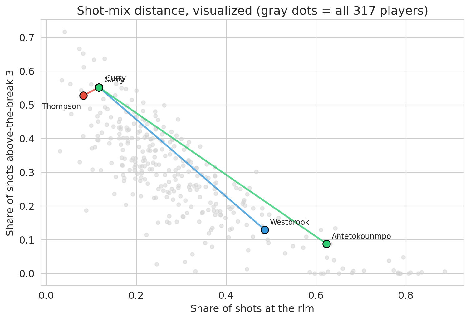
For shot mix, two players are "close" when their five shot-share percentages line up. The choice of distance is itself a value judgment. Euclidean distance on shot mix says two players are similar when their *recipes* match, regardless of height, defense, rebounding, or even total shot volume. A star and a role player who take the same proportions from each zone look identical to this metric.
The distances between famous pairs make the implications concrete:
```{python}
scaler = StandardScaler().fit(nba[features].values)

def shot_mix_distance(name1, name2):
    """Euclidean distance between two players in standardized shot-mix space."""
    v1 = scaler.transform(nba.loc[nba['PLAYER_NAME']==name1, features].values)[0]
    v2 = scaler.transform(nba.loc[nba['PLAYER_NAME']==name2, features].values)[0]
    return float(np.linalg.norm(v1 - v2))

pairs = [
    ('Stephen Curry', 'Klay Thompson'),         # both Warriors shooters (Klay has a notable midrange share)
    ('Stephen Curry', 'Buddy Hield'),           # both heavy three-point shooters
    ('Stephen Curry', 'Russell Westbrook'),     # both PGs, very different styles
    ('Stephen Curry', 'Giannis Antetokounmpo'), # guard vs interior force
    ('Nikola Jokić', 'Joel Embiid'),            # both All-NBA centers
    ('LeBron James', 'Kevin Durant'),           # both elite all-around scorers
]
for a, b in pairs:
    print(f"  d({a}, {b}) = {shot_mix_distance(a, b):.2f}")
```
Curry and Klay are nearly identical (both Warriors shooters). Curry and Hield are nearly as close — same role on different teams. Curry and Westbrook share a position label but sit far apart in shot-mix space. Curry and Giannis are at opposite ends of the map. Even Jokić and Embiid — both elite centers — are separated by a non-trivial distance: Embiid takes far more midrange shots, while Jokić lives in the paint. The position label hides these differences; shot mix exposes them.
```{python}
spotlight_pairs = [
    ('Stephen Curry', 'Klay Thompson', '#e74c3c'),
    ('Stephen Curry', 'Russell Westbrook', '#3498db'),
    ('Stephen Curry', 'Giannis Antetokounmpo', '#2ecc71'),
]

# Custom label offsets to avoid overlap. Curry and Klay sit on top of each
# other (the point of the figure!), so we push their labels in opposite
# directions; for other pairs the default upper-right offset is fine.
label_offsets = {
    # Curry and Klay sit on top of each other (that's the point); push Curry up-right
    # and Thompson down-left so the two labels don't collide.
    ('Stephen Curry', 'Klay Thompson'):      ((8, 8),  (-50, -16)),
    ('Stephen Curry', 'Russell Westbrook'):  ((6, 6),  (6, 6)),
    ('Stephen Curry', 'Giannis Antetokounmpo'): ((6, 6), (6, 6)),
}

fig, ax = plt.subplots(figsize=(8, 5.5))
ax.scatter(nba['pct_RA'], nba['pct_ATB3'], color='lightgray', alpha=0.5, s=20)

for a, b, col in spotlight_pairs:
    xa, ya = nba.loc[nba['PLAYER_NAME']==a, ['pct_RA','pct_ATB3']].values[0]
    xb, yb = nba.loc[nba['PLAYER_NAME']==b, ['pct_RA','pct_ATB3']].values[0]
    ax.plot([xa, xb], [ya, yb], color=col, linewidth=2, alpha=0.8)
    ax.scatter([xa, xb], [ya, yb], color=col, s=80, edgecolors='black', linewidths=1, zorder=3)
    oa, ob = label_offsets[(a, b)]
    ax.annotate(a.split()[-1], (xa, ya), xytext=oa, textcoords='offset points', fontsize=9)
    ax.annotate(b.split()[-1], (xb, yb), xytext=ob, textcoords='offset points', fontsize=9)

ax.set_xlabel('Share of shots at the rim')
ax.set_ylabel('Share of shots above-the-break 3')
ax.set_title('Shot-mix distance, visualized (gray dots = all 317 players)')
plt.tight_layout()
plt.show()
```
K-means uses exactly this distance. It groups players who sit close together in standardized shot-mix space, ignoring position, height, and volume. Every clustering algorithm inherits the similarity measure it is given. A clustering built on *salary* would group players differently; one built on *defensive stats* would too. The distance metric is the first place a value judgment enters the analysis.
## How k-means works
:::{.callout-important}
## Definition: Centroid
The **centroid** of a cluster is the mean of the feature vectors of the points assigned to it. For cluster $C_k$,
$$\mu_k = \frac{1}{|C_k|} \sum_{i \in C_k} x_i.$$
K-means represents each cluster by its centroid — a single point in feature space that summarizes the whole group.
:::
K-means is an iterative algorithm. We start by picking $k$ centroids and then repeat two steps until assignments stop changing:
1. **Initialize** $k$ centroids (randomly).
2. **Assign** each point to the nearest centroid.
3. **Recompute** each centroid as the mean of its assigned points.
Loop on steps 2-3 until no point changes its assignment.
:::{.callout-important}
## Definition: Sum of squared errors (SSE)
K-means minimizes the total within-cluster sum of squared distances from each point to its assigned cluster centroid — the **sum of squared errors (SSE)**:
$$\text{SSE} = \sum_{k=1}^{K} \sum_{i \in C_k} \|x_i - \mu_k\|^2$$
- $K$ is the number of clusters (chosen by us).
- $C_k$ is the set of data points assigned to cluster $k$.
- $x_i$ is the feature vector for data point $i$ (here, one player's shot-mix percentages).
- $\mu_k$ is the **centroid** of cluster $k$ — the mean of the points in $C_k$.
- $\|x_i - \mu_k\|^2$ is the squared Euclidean distance from point $i$ to its cluster's centroid.
:::
Every iteration decreases the SSE or leaves it unchanged, and the number of possible assignments is finite — so the algorithm must eventually stop changing the assignment and terminate. The objective is non-convex, so different starting points can converge to different **local optima**.
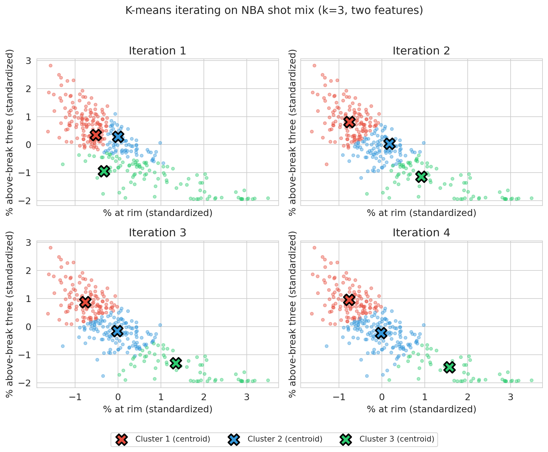
To visualize the iterations, we run the algorithm on just two features — `pct_RA` (share at the rim) and `pct_ATB3` (share above the break from three).
```{python}
np.random.seed(42)
X_viz = nba[['pct_RA', 'pct_ATB3']].values
X_viz_scaled = StandardScaler().fit_transform(X_viz)

# Initialize three centroids by picking three random players
k = 3
init_idx = np.random.choice(len(X_viz_scaled), size=k, replace=False)
centroids = X_viz_scaled[init_idx].copy()
```
Starting from these three random centroids, the cell below runs four iterations of assign-and-recompute, plotting the partition after each round so the centroids' drift toward stability is visible.
```{python}
fig, axes = plt.subplots(2, 2, figsize=(10, 8), sharex=True, sharey=True)
colors = ['#e74c3c', '#3498db', '#2ecc71']

for step in range(4):
    ax = axes[step // 2, step % 2]
    distances = np.array([np.sum((X_viz_scaled - c)**2, axis=1) for c in centroids])
    labels = distances.argmin(axis=0)
    for j in range(k):
        mask = labels == j
        ax.scatter(X_viz_scaled[mask, 0], X_viz_scaled[mask, 1],
                   c=colors[j], alpha=0.4, s=15)
        ax.scatter(centroids[j, 0], centroids[j, 1],
                   c=colors[j], marker='X', s=200, edgecolors='black', linewidths=2,
                   label=f'Cluster {j+1} (centroid)' if step == 0 else None)
    ax.set_xlabel('% at rim (standardized)')
    ax.set_ylabel('% above-break three (standardized)')
    ax.set_title(f'Iteration {step + 1}')
    for j in range(k):
        if (labels == j).sum() > 0:
            centroids[j] = X_viz_scaled[labels == j].mean(axis=0)

# Shared legend across all four panels (handles come from iteration 1)
handles, labels_legend = axes[0, 0].get_legend_handles_labels()
fig.legend(handles, labels_legend, loc='lower center', ncol=3,
           bbox_to_anchor=(0.5, -0.02), fontsize=10, frameon=True)
plt.suptitle('K-means iterating on NBA shot mix (k=3, two features)', fontsize=14, y=0.98)
plt.tight_layout(rect=[0, 0.04, 1, 0.96])
plt.show()
```
Panel 1 shows the random initial centroids and their first assignment; by panel 4 the centroids have stabilized and assignments barely change. K-means is simple and converges in a finite number of steps: the number of possible assignments is finite, and as long as the assignment changes from one iteration to the next, SSE strictly decreases — so the assignment must eventually stop changing, at which point the algorithm has converged. The solution is only a *local* optimum, an issue we return to below.
The two steps in the algorithm above are the two halves of an **alternating minimization** of SSE: step 2 fixes the centroids and re-assigns each point to its nearest one (the SSE-minimizing assignment); step 3 fixes the assignments and sets each centroid to the mean of its points (the SSE-minimizing centroid, and the source of the "mean" in k-means). The alternating-minimization pattern is the same engine that fits PCA in Chapter 14.
:::{.callout-note collapse="true"}
## Going deeper: k-means assumes round clusters
K-means assumes round clusters. The Euclidean-distance objective rewards solutions where each cluster is roughly spherical and similar in size. On data with elongated, curved, or non-convex clusters (think two interlocking crescents), k-means produces straight-line boundaries and misses the real structure. Spectral clustering and DBSCAN are common alternatives for shape-aware clustering — beyond our scope, but worth knowing they exist. Your features determine your clusters; your *algorithm* determines your cluster shapes.
:::
The two-feature view is for visualization only. The real archetypes appear when we cluster on all five zones at once.
## Discovering archetypes (k=5)
We standardize all five shot-mix features and fit k-means with $k=5$. The next section addresses how to *choose* $k$; for now we examine what $k=5$ returns.
```{python}
X_scaled = StandardScaler().fit_transform(nba[features].values)
kmeans_5 = KMeans(n_clusters=5, random_state=42, n_init=10)
raw_labels = kmeans_5.fit_predict(X_scaled)

def relabel_by_key(raw, df, key, ascending=False):
    """Remap cluster IDs so cluster 0 has the largest (or smallest) mean of `key`.

    Sklearn returns cluster labels in arbitrary order: change the random seed
    and the IDs shuffle. We sort by a meaningful statistic so that prose like
    "Archetype 0 = rim-heaviest group" stays true across runs and across
    sklearn versions."""
    means = df.groupby(raw)[key].mean()
    order = means.sort_values(ascending=ascending).index.tolist()
    remap = {old: new for new, old in enumerate(order)}
    return np.array([remap[r] for r in raw])

nba['archetype'] = relabel_by_key(raw_labels, nba, 'pct_RA', ascending=False)

profile = nba.groupby('archetype')[features].mean().round(2)
print(profile)
print(f"\nCluster sizes: {nba.groupby('archetype').size().to_dict()}")
```
Each row of the table is one archetype's average shot mix — a fingerprint. To check whether those averages capture a recognizable type, we list the six highest-volume players in each cluster.
```{python}
# Top-volume players per cluster — a sanity check that the archetypes are recognizable
for c in sorted(nba['archetype'].unique()):
    sample = nba[nba['archetype']==c].nlargest(6, 'FGA')['PLAYER_NAME'].tolist()
    print(f"Archetype {c}: {sample}")
```
:::{.callout-tip}
## Think about it
Before reading on, look at the cluster profiles and the top players. Can you give each archetype a one-word name? Which traditional positions (PG, SG, SF, PF, C) show up together in the same cluster?
:::
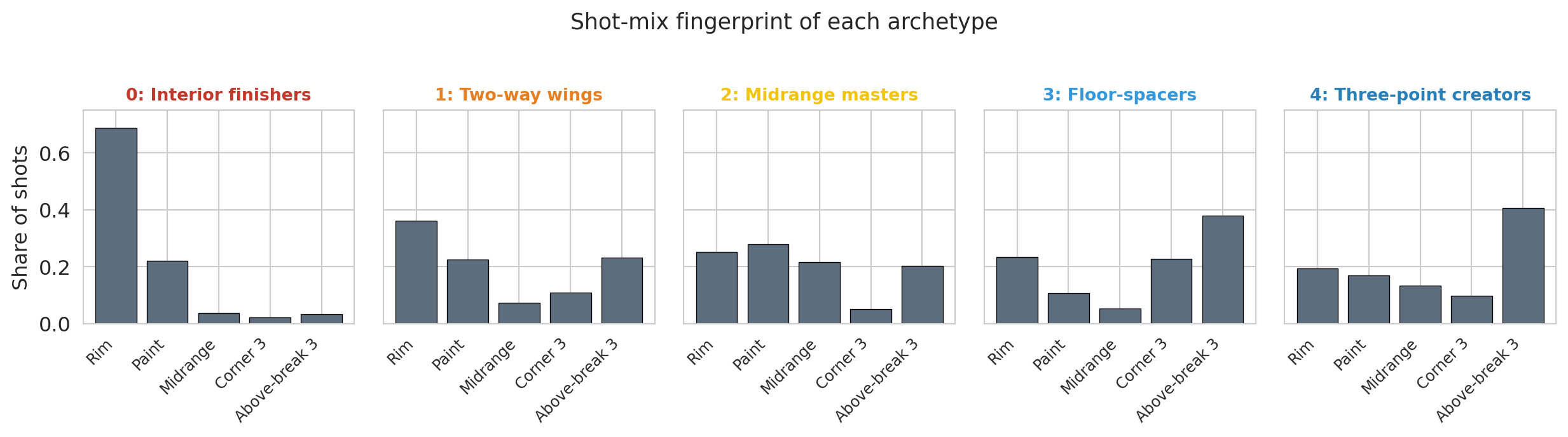
The five clusters correspond to recognizable modern archetypes. Reading the profile table from the most rim-heavy cluster to the least:
- **Archetype 0 — Interior finishers** (Giannis, Zion, Sabonis): overwhelming share at the rim, almost no threes. The bigs and downhill drivers who finish lobs, roll to the basket, and clean the glass.
- **Archetype 1 — Two-way wings** (LeBron, Kuzma, Jaylen Brown): balanced across all zones. Versatile attackers without a single specialty.
- **Archetype 2 — Midrange masters** (Brunson, Edwards, Durant): the highest midrange share of any cluster (~3× the league baseline), with comparable rates at the rim, in the paint, and from three. Midrange is the distinguishing feature. Classic iso scorers and pull-up artists.
- **Archetype 3 — Floor-spacers** (Hield, DiVincenzo, Strus): threes dominate (61% of attempts), with very little midrange. Specialists who spot up for a kickout.
- **Archetype 4 — Three-point creators** (Curry, Luka, Tatum): mostly above-the-break threes with some rim attempts. Guards who pull up off the dribble and finish at the basket.
The cluster numbering is not what k-means returned. Sklearn's cluster IDs are arbitrary: change the random seed and they shuffle. The `relabel_by_key` helper above sorts clusters by mean rim share (descending) so that archetype 0 is the most rim-heavy and archetype 4 is the least. Sorting by a meaningful key is a useful trick any time you want to talk about clusters by name.
K-means ignored traditional positions entirely. The midrange-masters cluster mixes a point guard (Brunson), a wing (Edwards), and Kevin Durant. The three-point creators include Curry, Luka, and Tatum regardless of listed position. Jokić, a center, joins the midrange operators. The taxonomy reflects *how* a player scores, not the number on the box score.
```{python}
# Canonical archetype palette — reused in every figure that colors by archetype.
archetype_names = ['Interior finishers', 'Two-way wings', 'Midrange masters',
                   'Floor-spacers', 'Three-point creators']
archetype_colors = ['#c0392b', '#e67e22', '#f1c40f', '#3498db', '#2980b9']

# Bar chart of cluster profiles — easier to read than the table above.
# The zone palette is intentionally neutral so it doesn't collide with the
# archetype colors used in subsequent figures.
zone_labels = ['Rim', 'Paint', 'Midrange', 'Corner 3', 'Above-break 3']
zone_colors = ['#5d6d7e'] * 5  # single neutral; archetype identity lives in the panel title

fig, axes = plt.subplots(1, 5, figsize=(13, 3.5), sharey=True)
for c, ax in zip(range(5), axes):
    means = nba[nba['archetype']==c][features].mean().values
    ax.bar(range(5), means, color=zone_colors, edgecolor='black', linewidth=0.5)
    ax.set_xticks(range(5))
    ax.set_xticklabels(zone_labels, rotation=45, ha='right', fontsize=9)
    ax.set_title(f'{c}: {archetype_names[c]}', fontsize=10,
                 color=archetype_colors[c], fontweight='bold')
    ax.set_ylim(0, 0.75)
    if c == 0:
        ax.set_ylabel('Share of shots')
plt.suptitle('Shot-mix fingerprint of each archetype', fontsize=13, y=1.02)
plt.tight_layout()
plt.show()
```
The five fingerprints look visibly different. Interior finishers are a single tall bar at the rim; floor-spacers and three-point creators show two tall bars on the right (the threes); midrange masters concentrate their shots on the left side of the floor.
```{python}
# Scatter: %-at-rim vs %-above-break-3, colored by archetype (same palette as above)
fig, ax = plt.subplots(figsize=(8, 5.5))
for c in sorted(nba['archetype'].unique()):
    mask = nba['archetype'] == c
    ax.scatter(nba.loc[mask, 'pct_RA'], nba.loc[mask, 'pct_ATB3'],
               color=archetype_colors[c], alpha=0.7, s=30, label=archetype_names[c])
ax.set_xlabel('Share of shots at the rim')
ax.set_ylabel('Share of shots above-the-break 3')
ax.set_title('Archetypes spread across the shot-mix plane')
ax.legend(loc='best', fontsize=8)
plt.tight_layout()
plt.show()
```
The scatter shows the archetypes occupy distinct regions of the shot-mix plane. Interior finishers sit in the lower right (high rim share, low above-break-3). Floor-spacers and three-point creators sit in the upper left (low rim share, high above-break-3). Midrange masters and two-way wings fill the middle.
Back to the Pacers' opening question: a wing who can "space the floor and attack closeouts" sits in the floor-spacer or three-point-creator clusters — Hield's own archetype and the one next to it. Once the front office accepts that this is the lens, the shortlist of candidates falls out of the partition.
And the Curry-vs-Westbrook question that opened the chapter? Both listed as point guards; the cluster places them at opposite ends of the map. Curry sits in three-point creators (over half his attempts are above-the-break threes), while Westbrook lands among the two-way wings — at the most rim-heavy edge of that cluster, taking a larger share at the rim (0.49) than any other point guard in the league and closer to Giannis territory than to any other "point guard." Same position label, opposite archetypes — the labels weren't tracking how the players actually score.
:::{.callout-note collapse="true"}
## Going deeper: the modern positional revolution
Cluster-based player taxonomies have a history in basketball analytics. Muthu Alagappan's 2012 MIT Sloan paper used **topological data analysis** (a different unsupervised method that builds a network of overlapping clusters) to argue for 13 player categories instead of 5. Kirk Goldsberry's *Sprawlball* (2019) documents the disappearance of the midrange shot and the rise of the three-pointer. Our k=5 analysis is a simplified version of the same exercise.
:::
## Choosing k
How did we know $k=5$ was right? We didn't. $k$ is a **choice**, not a discovery. Two heuristics help narrow the range.
:::{.callout-important}
## Definition: Elbow method
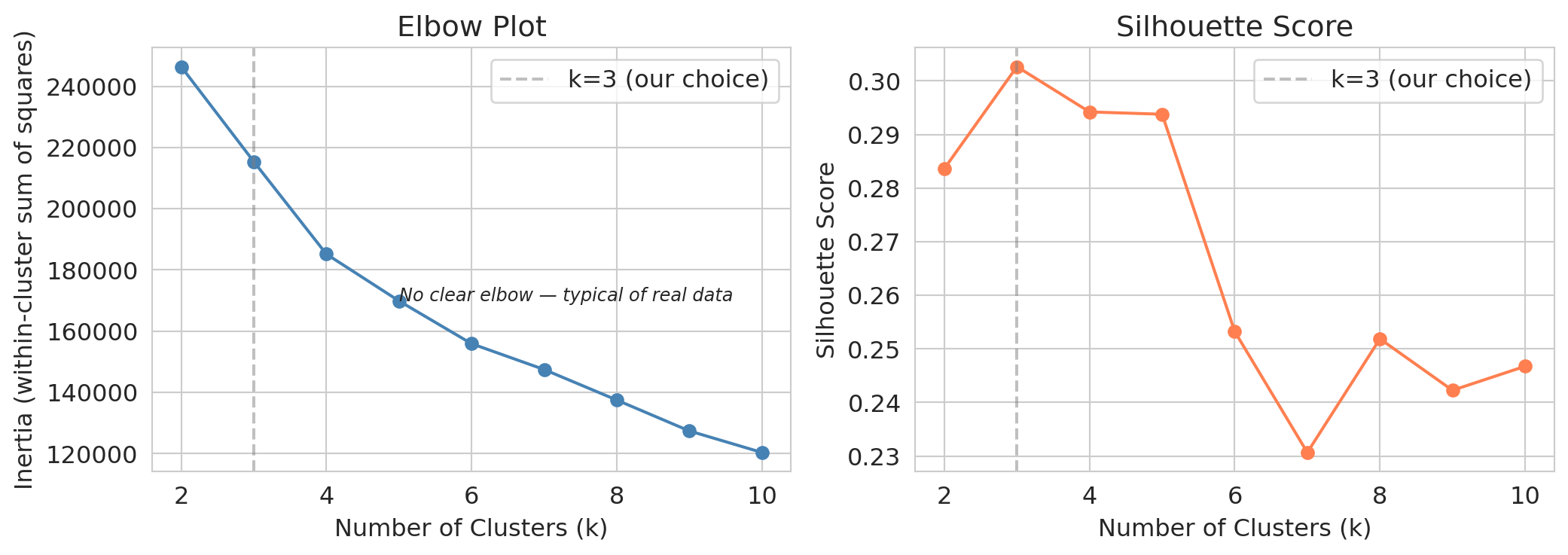
The **elbow method** plots the k-means SSE against the number of clusters $k$. SSE always decreases with $k$ — adding clusters can only reduce within-cluster distances — so the curve is monotone. The "elbow" is the value of $k$ beyond which adding clusters yields only small further reductions. Pick $k$ at the bend.
:::
The **silhouette score** is a second heuristic, worth a look even when it won't be the deciding voice.
:::{.callout-important}
## Definition: Silhouette score
The **silhouette score** measures how well each point fits its own cluster compared to the nearest other cluster.
For a point $x_i$ in cluster $C_k$, define
$$a(i) = \frac{1}{|C_k| - 1} \sum_{j \in C_k,\, j \ne i} \|x_i - x_j\|, \qquad b(i) = \min_{\ell \ne k} \frac{1}{|C_\ell|} \sum_{j \in C_\ell} \|x_i - x_j\|.$$
$a(i)$ is the mean distance from $x_i$ to other points in its cluster; $b(i)$ is the mean distance from $x_i$ to points in the nearest other cluster. The **silhouette of point $i$** is
$$s(i) = \frac{b(i) - a(i)}{\max(a(i), b(i))} \in [-1, 1].$$
The **silhouette score** is the mean of $s(i)$ across all points. Higher is better: $s(i) \approx 1$ means $x_i$ sits well inside its cluster; $s(i) \approx 0$ means it sits on a boundary; $s(i) < 0$ means it is closer to a different cluster than to its own.^[By convention, $s(i) = 0$ when $x_i$'s cluster contains only $x_i$ (so $a(i)$ would be a sum over an empty set). This matches sklearn's `silhouette_samples`.]
:::
```{python}
k_range = range(2, 11)
sses = []
silhouettes = []

for k in k_range:
    km = KMeans(n_clusters=k, random_state=42, n_init=10).fit(X_scaled)
    sses.append(km.inertia_)  # sklearn calls this `inertia_`; we label the quantity SSE
    silhouettes.append(silhouette_score(X_scaled, km.labels_))

fig, axes = plt.subplots(1, 2, figsize=(11, 4))

axes[0].plot(list(k_range), sses, 'o-', color='steelblue')
axes[0].axvline(x=5, color='gray', linestyle='--', alpha=0.5, label='k=5 (our choice)')
axes[0].set_xlabel('Number of clusters (k)')
axes[0].set_ylabel('SSE (within-cluster sum of squared distances)')
axes[0].set_title('Elbow plot')
axes[0].legend()

axes[1].plot(list(k_range), silhouettes, 'o-', color='coral')
axes[1].axvline(x=5, color='gray', linestyle='--', alpha=0.5, label='k=5 (our choice)')
axes[1].set_xlabel('Number of clusters (k)')
axes[1].set_ylabel('Silhouette score')
axes[1].set_title('Silhouette score (higher is better ↑)')
# Anchor at 0 so the visible gap between k=3 and k=5 reflects its true magnitude
# (~0.03 on a 0-to-1 scale) rather than being inflated by an auto-zoomed axis.
axes[1].set_ylim(0, 0.5)
axes[1].annotate('higher\nis better', xy=(0.97, 0.97), xycoords='axes fraction',
                 ha='right', va='top', fontsize=10,
                 bbox=dict(boxstyle='round,pad=0.3', fc='#fff7e6', ec='gray', lw=0.5))
axes[1].legend(loc='lower left')

plt.tight_layout()
plt.show()
```
Neither plot gives a definitive answer. The elbow is gradual, with no sharp bend. The silhouette score *peaks at $k=3$, with $k=2$ close behind*, then drifts down from there. Taken at face value, the silhouette recommends a coarse partition that would lump Curry, LeBron, and Brunson into the same group.
:::{.callout-tip}
## Think about it
The silhouette score peaks at $k=3$ (with $k=2$ close behind). We picked $k=5$. What information did we use that the silhouette score does not see?
:::
The heuristics rule out clearly bad choices ($k=20$ over-segments; $k=2$ under-segments) but cannot identify the granularity a particular task needs.
**The level of detail required to find a Hield replacement is not in the data — it is in the question the Pacers are asking.** We pick $k=5$ because the front office needs archetype-level resolution, finer than the silhouette score alone would recommend.
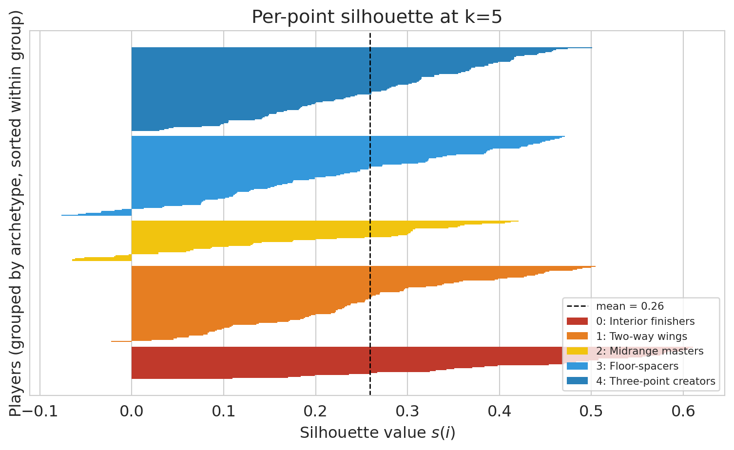
Each player gets their own silhouette value. The bars below show the full distribution at k=5: tall bars sit comfortably inside their cluster; thin or negative bars are boundary cases. The boundary-heavy archetypes are the ones we'll see flip across seeds in §How stable below.
```{python}
from sklearn.metrics import silhouette_samples

# Re-use the same relabeling as §Discovering archetypes so the colors and
# numbers below match the chapter's canonical archetype palette.
sil = silhouette_samples(X_scaled, nba['archetype'].values)

fig, ax = plt.subplots(figsize=(8, 5))
y_lower = 0
for c in range(5):
    vals = np.sort(sil[nba['archetype'].values == c])
    y_upper = y_lower + len(vals)
    ax.barh(np.arange(y_lower, y_upper), vals,
            color=archetype_colors[c], edgecolor='none', height=1.0,
            label=f'{c}: {archetype_names[c]}')
    y_lower = y_upper + 5  # small gap between archetypes
ax.axvline(sil.mean(), color='black', linestyle='--', linewidth=1,
           label=f'mean = {sil.mean():.2f}')
ax.set_xlabel('Silhouette value $s(i)$')
ax.set_ylabel('Players (grouped by archetype, sorted within group)')
ax.set_title('Per-point silhouette at k=5')
ax.set_yticks([])
ax.legend(loc='lower right', fontsize=8)
plt.tight_layout()
plt.show()
```
## Hierarchical clustering: don't commit to k up front
When the right $k$ is unclear, an alternative is to avoid choosing $k$ at all. **Hierarchical clustering** builds a *tree* of merges instead of a flat partition; we read off a clustering at any granularity afterwards.
The agglomerative algorithm:
1. **Start** with every point as its own cluster ($n$ clusters total).
2. **Merge** the two closest clusters into one.
3. **Repeat** until a single cluster remains.
The result is a **dendrogram**, a tree whose leaves are individual players and whose root is the full dataset. Cutting the tree at a chosen height yields a clustering at the corresponding granularity.
The algorithm needs a definition of distance between two *clusters*, not just two points. The choice is called a **linkage rule**. Common options:
- **Single linkage**: distance between two clusters is the minimum pairwise distance — produces long, stringy clusters.
- **Complete linkage**: maximum pairwise distance — produces compact, ball-shaped clusters.
- **Average linkage**: mean pairwise distance.
- **Ward**: merges the pair whose union increases the total SSE by the least.
We use **Ward** for the rest of this chapter because it is the rule most consistent with the k-means objective — both minimize SSE. The other three rules belong on the menu (they show up in advanced clustering courses and they produce visibly different dendrograms on the same data), but we won't return to them here. Trying several linkage rules on a new dataset is a useful sensitivity check.
```{python}
from scipy.cluster.hierarchy import linkage, dendrogram, fcluster

Z = linkage(X_scaled, method='ward')

fig, ax = plt.subplots(figsize=(10, 4.5))
dendrogram(Z, truncate_mode='lastp', p=30, no_labels=True,
           color_threshold=Z[-4, 2], above_threshold_color='gray', ax=ax)
ax.axhline(y=Z[-3, 2], color='black', linestyle='--', alpha=0.5)
ax.axhline(y=Z[-5, 2], color='black', linestyle='--', alpha=0.5)
ax.text(0.02, Z[-3, 2], ' cut at k=3', va='bottom', ha='left', fontsize=10,
        transform=ax.get_yaxis_transform())
ax.text(0.02, Z[-5, 2], ' cut at k=5', va='bottom', ha='left', fontsize=10,
        transform=ax.get_yaxis_transform())
ax.set_xlabel('Players (last 30 merges shown)')
ax.set_ylabel('Linkage distance (Ward)')
ax.set_title('Hierarchical clustering of NBA players by shot mix')
plt.tight_layout()
plt.show()
```
The dendrogram shows the cluster structure at every granularity simultaneously. The upper dashed line cuts the tree into three groups; the lower one into five. A lower cut produces a finer partition.
```{python}
# Cut the tree to get k=5 clusters. fcluster labels are 1..k; we 0-index for consistency.
hier_labels = fcluster(Z, t=5, criterion='maxclust') - 1

# Relabel by rim share, same trick we used for k-means
nba['archetype_hier'] = relabel_by_key(hier_labels, nba, 'pct_RA', ascending=False)

print("Hierarchical k=5 cluster profiles:")
print(nba.groupby('archetype_hier')[features].mean().round(2))
print()
ari_km_vs_hier = adjusted_rand_score(nba['archetype'], nba['archetype_hier'])
print(f"ARI between k-means k=5 and hierarchical k=5: {ari_km_vs_hier:.2f}")
```
The two methods disagree on some boundary players but agree on the broad archetype structure. The interior-finisher / floor-spacer split appears under both algorithms. Agreement across algorithms is evidence that the structure lives in the data, not in any single method.
Hierarchical clustering is slower than k-means: it stores all pairwise distances (memory grows with the *square* of the number of points $n$) and runs in time that grows much faster than linearly with $n$, compared to k-means' near-linear cost per iteration. Both costs become impractical for very large $n$. For hundreds or low thousands of points where $k$ is unknown, hierarchical clustering is a useful complement — inspect the tree first, then choose a cut.
## How stable are these clusters?
Before we ask what *other* features could change the answer, let's ask how stable the answer is to a smaller perturbation: the random seed. K-means starts from random initial centroids. Different starts can yield different final partitions: the algorithm finds a **local optimum**, not the global one.
:::{.callout-tip}
## Think about it
If we re-ran k-means with different starting points, would the five archetypes survive? Would the *boundaries* shift? Which players would change cluster most often?
:::
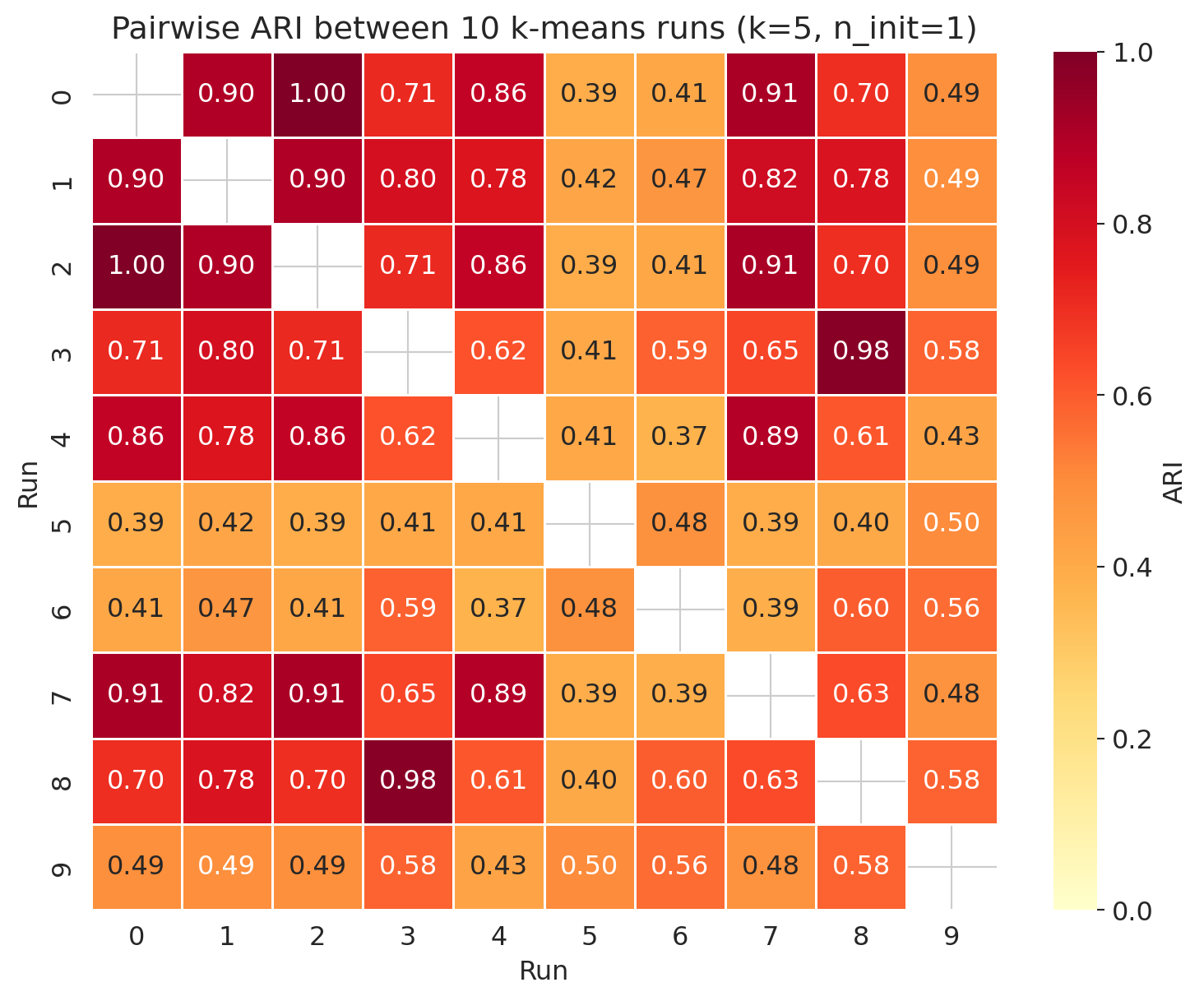
To expose the instability we run k-means 10 times with different seeds, each using just *one* random start per run (`n_init=1`). To compare two clusterings we use the **Adjusted Rand Index (ARI)**.
:::{.callout-important}
## Definition: Adjusted Rand Index (ARI)
The **Adjusted Rand Index** measures agreement between two clusterings of the same points, corrected for the agreement expected by chance. Across all pairs of points, the ARI asks whether the two clusterings agree on whether each pair lands in the same cluster.
- $\mathrm{ARI} = 1$: perfect agreement.
- $\mathrm{ARI} = 0$: agreement no better than chance.
- $\mathrm{ARI} < 0$: the two clusterings disagree *more* than chance would predict (rare but possible).
:::
```{python}
# Run k-means 10 times with different random seeds
all_labels = []
for seed in range(10):
    km = KMeans(n_clusters=5, random_state=seed, n_init=1)
    all_labels.append(km.fit_predict(X_scaled))

ari_matrix = np.zeros((10, 10))
for i in range(10):
    for j in range(10):
        ari_matrix[i, j] = adjusted_rand_score(all_labels[i], all_labels[j])

fig, ax = plt.subplots(figsize=(8, 6.5))
display_matrix = ari_matrix.copy()
np.fill_diagonal(display_matrix, np.nan)
sns.heatmap(display_matrix, annot=True, fmt='.2f', cmap='YlOrRd',
            ax=ax, vmin=0, vmax=1, cbar_kws={'label': 'ARI'},
            linewidths=0.5, linecolor='white')
ax.set_xlabel('Run')
ax.set_ylabel('Run')
ax.set_title('Pairwise ARI between 10 k-means runs (k=5, n_init=1)')
plt.tight_layout()
plt.show()

off_diag = ari_matrix[np.triu_indices(10, k=1)]
print(f"ARI mean: {off_diag.mean():.3f}")
print(f"ARI range: {off_diag.min():.3f} to {off_diag.max():.3f}")
```
The mean ARI is moderate and the spread is wide. Some seed-pairs produced exactly the same partition (ARI = 1.0) — those starts converged to identical local optima — while others agreed only weakly. The archetypes are partially stable; the boundaries are not. Some players flip groups depending on the seed.
```{python}
# Which players sit at archetype boundaries?
# Sklearn returns labels in arbitrary order per run, so we re-apply the
# rim-share-sort relabeling to each run before comparing to the baseline.
# That way `flips` counts true partition disagreement, not label-ID shuffles.
baseline = nba['archetype'].values
boundary_counts = np.zeros(len(nba), dtype=int)
for raw in all_labels:
    aligned = relabel_by_key(raw, nba, 'pct_RA', ascending=False)
    boundary_counts += (aligned != baseline).astype(int)

nba_boundary = nba.copy()
nba_boundary['flips'] = boundary_counts
boundary_players = nba_boundary[nba_boundary['FGA'] >= 800].nlargest(8, 'flips')[['PLAYER_NAME', 'flips']]
print("High-volume players whose archetype is least stable across seeds:")
print(boundary_players.to_string(index=False))
```
The boundary-flippers are not noise; they are information. A player who sits between two archetypes is a hybrid, and the instability of the clustering reveals what the rigid k=5 labels cannot.
So what do practitioners do about this? Throughout the rest of the chapter we pass `n_init=10` explicitly so k-means picks the best of 10 starts — recent sklearn versions default `n_init` to `'auto'`, which resolves to 1 under the default `k-means++` initializer, so a bare `KMeans(...)` call gives you a single random start. Sklearn also defaults to **k-means++ initialization**: instead of picking starting centroids uniformly at random, k-means++ picks the first centroid at random and then each subsequent centroid with probability proportional to its squared distance from the centroids already chosen — biasing the starts to be spread apart. The combination — k-means++ plus `n_init=10` — is what makes k-means usable in practice; it mitigates the local-optimum problem but does not guarantee identical clusters across calls.
**In practice: always pass `n_init=10` to k-means, and use the default `k-means++` initializer.** These reduce sensitivity to the random start; the diagnostic above shows what happens when you don't use them. For figures and prose that need to match across runs, also fix a `random_state` — that's what guarantees reproducibility, not the tricks.
:::{.callout-note collapse="true"}
## Going deeper: validating clustering with held-out data
We measured stability across random seeds. A complementary check borrows from Chapter 6: split the players into training and test sets, fit k-means on training, then assign each test player to the nearest training centroid. If the test reconstruction error is comparable to the training reconstruction error, the clusters generalize beyond the training sample. This is the same logic that validated PCA via held-out reconstruction in Chapter 14.
:::
## Your features determine your clusters
Seed instability tells us where the boundaries of our k=5 partition sit. A bigger question is whether the same 317 players, *clustered on different features entirely*, even land in the same neighborhoods at all. The five archetypes are not the *only* way to cluster these players. Same algorithm, same players, different feature set, different answer. Two alternative feature recipes illustrate the point.
### Cluster on shot *volume* (total attempts)
For volume, we cluster on a single feature: total field goal attempts. K-means on a one-dimensional feature reduces to grouping players by how many shots they take, with each cluster a contiguous range of FGA counts — a slightly fancier version of sorting players and splitting them into five tiers (the algorithm picks the four cut-points that minimize within-cluster squared error).
```{python}
X_vol = StandardScaler().fit_transform(nba[['FGA']].values)
raw_vol = KMeans(n_clusters=5, random_state=42, n_init=10).fit_predict(X_vol)
nba['cluster_vol'] = relabel_by_key(raw_vol, nba, 'FGA', ascending=False)

for c in sorted(nba['cluster_vol'].unique()):
    sub = nba[nba['cluster_vol']==c]
    sample = sub.nlargest(4, 'FGA')['PLAYER_NAME'].tolist()
    print(f"Volume tier {c} (FGA range {sub['FGA'].min():.0f}–{sub['FGA'].max():.0f}): {sample}")
```
The volume clusters form a clean ladder: tier 0 holds the league's highest-volume scorers, tier 4 the bench players who barely cleared the 200-FGA cutoff. The structure captures one signal, total shots taken. Players with very different shot mixes (Luka and Brunson, say) end up together if they take similar numbers of shots.
### Cluster on shot *efficiency* (effective FG%)
For efficiency we use **effective field-goal percentage** (eFG%): standard FG%, but each made three-pointer counts as 1.5 makes to reflect its higher point value. The metric is the NBA's standard "shooting efficiency" statistic and compares a three-point shooter to a rim finisher on a common scale.
```{python}
nba['fgm_total'] = nba[['RA_FGM','PAINT_FGM','MID_FGM','LC3_FGM','RC3_FGM','ATB3_FGM']].sum(axis=1)
nba['3pm']       = nba[['LC3_FGM','RC3_FGM','ATB3_FGM']].sum(axis=1)
nba['efg_pct']   = (nba['fgm_total'] + 0.5 * nba['3pm']) / nba['FGA']

X_eff = StandardScaler().fit_transform(nba[['efg_pct']].values)
raw_eff = KMeans(n_clusters=5, random_state=42, n_init=10).fit_predict(X_eff)
nba['cluster_eff'] = relabel_by_key(raw_eff, nba, 'efg_pct', ascending=False)

for c in sorted(nba['cluster_eff'].unique()):
    sub = nba[nba['cluster_eff']==c]
    sample = sub.nlargest(4, 'FGA')['PLAYER_NAME'].tolist()
    print(f"Efficiency tier {c} (eFG% range {sub['efg_pct'].min():.3f}–{sub['efg_pct'].max():.3f}): {sample}")
```
Another clean ladder, this time ordered by *skill*. Tier 0 holds the most efficient shooters in the league — rim finishers and rebounders who rarely miss. Tier 4 holds the players shooting well below league average (max 0.503; the 2023-24 NBA league-average eFG% was around 0.546). A high-volume but inefficient player (volume tier 0, efficiency tier 4) and a low-volume but accurate one (volume tier 4, efficiency tier 0) sit far apart in these clusterings even when they share a shot-mix archetype.
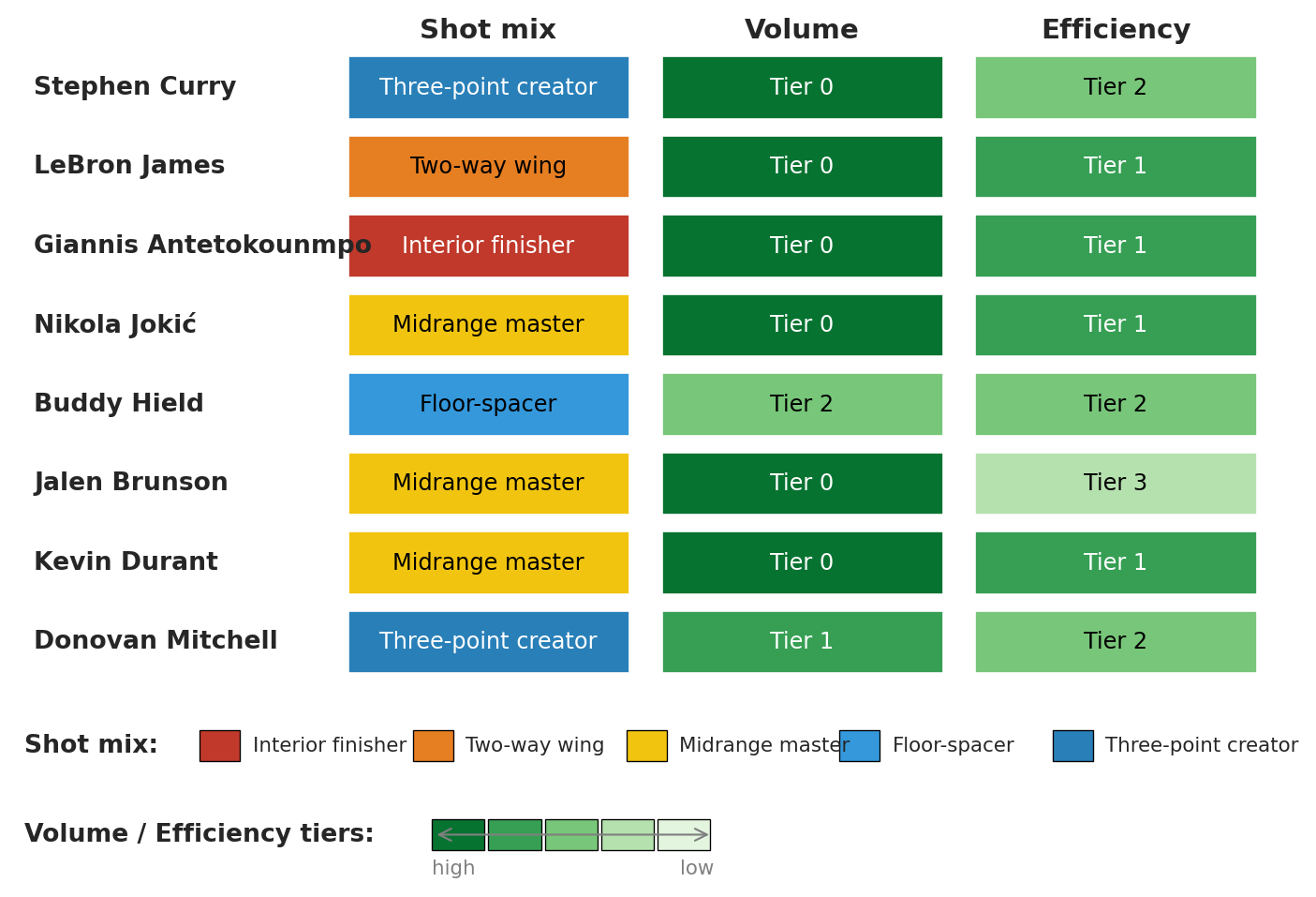
### Same players, three stories
Raw cluster IDs are arbitrary even after relabeling. We display each spotlight player's *named* label under all three clusterings, with color encoding the tier:
```{python}
#| code-fold: true
# Presentation figure — the takeaway is in the output, not the code.
# Singular form of archetype names for use in cells (matches archetype_colors above)
arch_names_singular = ['Interior finisher', 'Two-way wing', 'Midrange master',
                       'Floor-spacer', 'Three-point creator']
# Shared sequential palette for volume/efficiency tiers: dark=high, light=low
tier_palette = plt.get_cmap('Greens')
tier_colors = [tier_palette(0.85 - 0.18*i) for i in range(5)]

def text_color_for(rgba):
    """Choose black or white text based on background luminance (Rec. 601)."""
    r, g, b = rgba[:3]
    luma = 0.299*r + 0.587*g + 0.114*b
    return 'white' if luma < 0.5 else 'black'

import matplotlib.colors as mcolors  # for hex -> RGBA conversion
arch_rgba = [mcolors.to_rgba(c) for c in archetype_colors]

spotlight = ['Stephen Curry', 'LeBron James', 'Giannis Antetokounmpo',
             'Nikola Jokić', 'Buddy Hield', 'Jalen Brunson',
             'Kevin Durant', 'Donovan Mitchell']

fig = plt.figure(figsize=(9, 6))
gs = fig.add_gridspec(2, 1, height_ratios=[5, 1.4], hspace=0.05)
ax = fig.add_subplot(gs[0])
ax_leg = fig.add_subplot(gs[1])

ax.set_xlim(-0.5, 3.5)
ax.set_ylim(-0.5, len(spotlight)-0.5)
ax.invert_yaxis()

for row_i, name in enumerate(spotlight):
    row = nba[nba['PLAYER_NAME'] == name].iloc[0]
    a, v, e = row['archetype'], row['cluster_vol'], row['cluster_eff']
    ax.text(-0.45, row_i, name, va='center', ha='left', fontsize=10, fontweight='bold')
    for col_i, (label, rgba) in enumerate([
        (arch_names_singular[a], arch_rgba[a]),
        (f'Tier {v}',            tier_colors[v]),
        (f'Tier {e}',            tier_colors[e]),
    ]):
        ax.add_patch(plt.Rectangle((col_i + 0.55, row_i - 0.4), 0.9, 0.8,
                                   facecolor=rgba, edgecolor='white', linewidth=1))
        ax.text(col_i + 1.0, row_i, label, va='center', ha='center',
                fontsize=9, color=text_color_for(rgba))

for col_i, header in enumerate(['Shot mix', 'Volume', 'Efficiency']):
    ax.text(col_i + 1.0, -0.55, header, va='bottom', ha='center',
            fontsize=11, fontweight='bold')

ax.set_axis_off()

# Legend pane: archetype color swatches + tier color ramp
ax_leg.set_xlim(0, 10)
ax_leg.set_ylim(0, 4)
ax_leg.set_axis_off()

# Archetype swatches (one row): label "Shot mix" then five name+swatch pairs
ax_leg.text(0.05, 3.0, 'Shot mix:', va='center', ha='left',
            fontsize=10, fontweight='bold')
for i, (name, rgba) in enumerate(zip(arch_names_singular, arch_rgba)):
    x0 = 1.45 + 1.7 * i
    ax_leg.add_patch(plt.Rectangle((x0, 2.65), 0.32, 0.7,
                                   facecolor=rgba, edgecolor='black', linewidth=0.5))
    ax_leg.text(x0 + 0.42, 3.0, name, va='center', ha='left', fontsize=8)

# Tier color ramp: label "Volume / Efficiency tiers:" then 5-block gradient
ax_leg.text(0.05, 1.0, 'Volume / Efficiency tiers:', va='center', ha='left',
            fontsize=10, fontweight='bold')
for i, rgba in enumerate(tier_colors):
    x0 = 3.3 + 0.45 * i
    ax_leg.add_patch(plt.Rectangle((x0, 0.65), 0.42, 0.7,
                                   facecolor=rgba, edgecolor='black', linewidth=0.5))
ax_leg.annotate('', xy=(5.55, 1.0), xytext=(3.3, 1.0),
                arrowprops=dict(arrowstyle='<->', color='gray', lw=0.8))
ax_leg.text(3.3, 0.25, 'high', va='center', ha='left', fontsize=8, color='gray')
ax_leg.text(5.55, 0.25, 'low', va='center', ha='right', fontsize=8, color='gray')

plt.tight_layout()
plt.show()
```
Curry and Brunson share the top volume tier but split on shot mix and on efficiency. Jokić and Giannis sit one archetype apart but agree on volume and efficiency. Each row describes the same player three ways; none of the three descriptions is privileged.
How big is the disagreement? ARI puts a number on it.
```{python}
mix_labels = nba['archetype'].values
vol_labels = nba['cluster_vol'].values
eff_labels = nba['cluster_eff'].values

print(f"ARI(shot-mix, volume)      = {adjusted_rand_score(mix_labels, vol_labels):.3f}")
print(f"ARI(shot-mix, efficiency)  = {adjusted_rand_score(mix_labels, eff_labels):.3f}")
print(f"ARI(volume, efficiency)    = {adjusted_rand_score(vol_labels, eff_labels):.3f}")
```
All three pairwise ARIs land near zero — the volume-vs-efficiency pair is even slightly *negative*, meaning two analysts running the same algorithm on the same 317 players with different feature recipes would disagree on cluster membership *more* than two analysts running different random seeds. Recall §How stable: the cross-seed ARI mean was about 0.6. Feature choice scrambles the partition by roughly an order of magnitude more than the seed does.
A GM looking for a Buddy Hield replacement wants shot-mix archetypes — they identify players who fill the same *role*. A GM ranking trade targets by raw production should cluster on volume. A GM valuing a contract should cluster on efficiency. The feature choice follows the decision the GM needs to make.
:::{.callout-warning}
## Pick the features that match your decision
There is no "true" clustering of NBA players. Each feature recipe answers a different question. **Shot mix** asks "what kind of shots?" — gives archetypes. **Shot volume** asks "how many?" — gives stars-vs-role-players. **Shot efficiency** asks "how well?" — gives skill tiers. The feature choice is your responsibility — and it is also your liability when the decision has stakes.
:::
So far we've used clustering as a discovery tool on one dataset. The shot-mix archetypes were one possible answer to one possible question; volume tiers and skill tiers answered different questions; none was the "true" partition of the league. The same algorithm runs on cells, patients, and stars. Whether the clusters it returns deserve trust depends on what you can check *outside* the clustering itself.
---
## Clustering in the wild
The basketball half showed how feature choice shapes clusters when stakes are merely competitive. Four published studies turn on the same point at higher stakes — single-cell biology, asthma, depression, and stellar astronomy. Two succeeded, one failed cautionarily, one came out mixed.
### PCA, then k-means: a common recipe in the wild
K-means uses Euclidean distance, which behaves badly in high dimensions. With many features, correlated columns, or columns on different scales, distances become noisy and uninformative. The fix that dominates the wild is to run PCA first and then k-means on the PC scores — Euclidean distance is much more trustworthy in the reduced space.
The standard recipe:
1. **Standardize** the features so no single column dominates the distance calculation.
2. **PCA** down to $k$ components, picked from a scree plot or the elbow ([Chapter 14](lec14-pca.qmd)).
3. **K-means** on the $k$-dimensional PC scores.
The recipe has variants. At larger scales — millions of cells, for example — the k-means step is often swapped for a graph-based clusterer (community detection on a $k$-nearest-neighbor graph), but the dimension-reduction logic is identical; Tabula Muris below is that variant. Some pipelines skip PCA when the feature count is small enough that distances stay meaningful in the raw space (Haldar). Some replace PCA with a dimension-reduction step that uses *both* the features and an auxiliary signal (Drysdale's CCA), which carries its own dangers — see that case study. The four studies below illustrate where the recipe works, where it breaks, and what swaps preserve its validity.
### Tabula Muris: clustering as the scaffolding of a cell atlas
The Tabula Muris Consortium profiled the gene expression of 100,605 individual cells across 20 mouse organs.[^tabula-muris] No cell came pre-labeled with its type. Their pipeline ran in two stages. First, select a few thousand highly variable genes and run PCA on those to reduce each cell's expression vector to a few dozen components. Then cluster the cells with a graph-based community-detection algorithm — Louvain, packaged in the standard single-cell toolkit Seurat — by building a $k$-nearest-neighbor graph on the PC scores and finding densely connected groups. The result was up to around 50 clusters per organ.
The use was a *good* one. Each cluster was annotated against known **marker genes** — genes that decades of cell-biology research had already pinned to specific cell types. When a cluster's top-expressed genes lined up with the marker set for, say, hepatocytes, the cluster got that name. Almost every named cell type in mouse anatomy came back out. The clustering itself didn't reveal cell types; it organized the data well enough that biologists could verify each group against an existing standard.
{fig-align="center" width="80%"}
[^tabula-muris]: Tabula Muris Consortium (2018). Single-cell transcriptomics of 20 mouse organs creates a *Tabula Muris*. *Nature* 562, 367–372. <https://www.nature.com/articles/s41586-018-0590-4>.
### Haldar: clusters that change which drug you should take
Haldar and colleagues clustered three asthma cohorts on 8 clinical and physiologic features:[^haldar] age of asthma onset; sex; **atopic** status (whether the patient is prone to allergic reactions); body-mass index; peak-flow variability; **FEV1** bronchodilator response (forced expiratory volume in one second — the standard lung-function measurement); **sputum eosinophil** count (eosinophils are immune cells whose presence in coughed-up airway secretions signals allergic-type inflammation); and exhaled nitric oxide.
Three cohorts ran through the analysis: a primary-care sample (n = 184), a refractory secondary-care sample (n = 187), and a longitudinal randomized trial (n = 68). The method ran in two stages — Ward's hierarchical clustering (a bottom-up agglomerative algorithm) on the first cohort to pick $k$, then k-means with that $k$ for the analysis on the subsequent cohorts.
Two clusters showed up in both the primary-care and the refractory cohorts: **early-onset atopic** asthma and **obese non-eosinophilic** asthma. Two additional clusters appeared only in the refractory cohort and were *discordant* — symptoms and inflammation moved in opposite directions. A **symptom-predominant** group had many symptoms but little eosinophilic inflammation; an **inflammation-predominant** group had eosinophilic inflammation but few symptoms.
The validation was a randomized trial. Patients in the inflammation-predominant cluster were assigned either to management by symptoms (the standard of care) or to management by inflammation markers. The inflammation-managed arm cut exacerbations from roughly 3.5 to 0.4 per patient per year. Symptom-predominant patients managed by symptoms received substantially less inhaled steroid than they would have under inflammation-marker management. Cluster membership predicted *which treatment helped which patient* — a harder test than "the clusters look biologically interpretable." Different treatments worked in different clusters, so the clusters mapped onto a real joint in the disease.
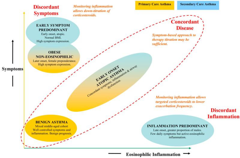{fig-align="center" width="80%"}
[^haldar]: Haldar, P., Pavord, I. D., Shaw, D. E., et al. (2008). Cluster analysis and clinical asthma phenotypes. *American Journal of Respiratory and Critical Care Medicine* 178, 218–224. <https://www.atsjournals.org/doi/10.1164/rccm.200711-1754OC>.
### Drysdale: beautiful clusters, no replication
Drysdale and colleagues claimed to discover **four biotypes of depression** in 2017.[^drysdale] Their pipeline ran canonical correlation analysis (CCA — a method for finding linear combinations of two feature sets that correlate maximally) on resting-state fMRI (functional MRI) connectivity features and clinical symptom scores from 1,188 patients, then hierarchical clustering on the CCA-projected fMRI scores. The authors reported that the four biotypes were diagnosable from fMRI alone with 82–93% sensitivity and specificity and that they predicted response to transcranial magnetic stimulation (TMS) therapy.
Two years later, Dinga and colleagues attempted to replicate the pipeline on an independent sample of 187 patients.[^dinga] The replication tests came in three layers, all consistent. First, under a null of no association between the two feature sets, permutation tests on the canonical correlations returned p-values of 0.64 and 0.99 — well above any reasonable threshold. Second, the canonical correlations recomputed on held-out data — a CCA-specific analog of the train/test split from Chapter 6 — dropped to about zero, so Drysdale's correlations did not generalize. Third, under a null of no cluster structure, both the Calinski-Harabasz statistic (a between-vs-within cluster scatter ratio) and the silhouette score returned non-significant p-values (0.45 and 0.19) — the four-cluster solution was no better than chance. And leaving one subject out at a time changed cluster assignments for a substantial fraction of subjects, far more than a stable clustering would produce.
The mechanism is general. CCA can always find linear combinations of two high-dimensional feature sets that look correlated *in the data they were fit on*, even when no relationship exists in the population. With enough features and not enough samples — the features-to-samples ratio Drysdale ran is far into that regime — the optimization step *manufactures* apparent structure. Without a permutation test or out-of-sample replication, that manufactured structure cannot be distinguished from a real signal. Drysdale's original analysis ran neither step. Dinga's ran both, and the structure dissolved.
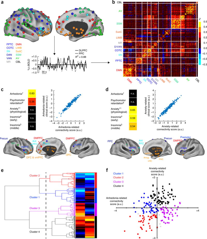{fig-align="center" width="80%"}
[^drysdale]: Drysdale, A. T., Grosenick, L., Downar, J., et al. (2017). Resting-state connectivity biomarkers define neurophysiological subtypes of depression. *Nature Medicine* 23, 28–38. <https://www.nature.com/articles/nm.4246>.
[^dinga]: Dinga, R., Schmaal, L., Penninx, B. W. J. H., et al. (2019). Evaluating the evidence for biotypes of depression: methodological replication and extension of Drysdale et al. (2017). *NeuroImage: Clinical* 22, 101796. <https://www.sciencedirect.com/science/article/pii/S2213158219302827>.
### APOGEE: the same lesson, in physics
Garcia-Dias and colleagues ran k-means on 153,847 stellar spectra from the APOGEE survey — the Apache Point Observatory Galactic Evolution Experiment, a high-resolution near-infrared spectroscopic survey of Milky Way stars.[^garcia-dias] The input features were the normalized flux at each wavelength — the raw spectra — not derived astrophysical parameters like temperature, surface gravity, or metallicity.
The result came out mixed. Some broad stellar-population classes were recovered: high-luminosity giants vs. low-luminosity dwarfs, substructure within the giant branch, and an inner-galaxy vs. outer-galaxy split. But the recovery was partial, the algorithm was sensitive to initialization, and the authors flagged the core limitation themselves: *"a discrete classification in flux space does not result in a neat organisation in the parameters' space."*
The underlying objects — distinct stellar populations differing in mass, age, and chemical composition — are physically real. Yet k-means in raw-flux space only partially recovered them, because Euclidean distance between two spectra is not the same notion of similarity as distance between two stars in the parameter space astronomers actually care about. The clustering algorithm did its job correctly; the *similarity metric* — encoded by the feature choice — was the wrong one for the question.
{fig-align="center" width="80%"}
[^garcia-dias]: Garcia-Dias, R., Allende Prieto, C., Sánchez Almeida, J., & Ordovás-Pascual, I. (2018). Machine learning in APOGEE: unsupervised spectral classification with $K$-means. *Astronomy & Astrophysics* 612, A98. <https://www.aanda.org/articles/aa/full_html/2018/04/aa32134-17/aa32134-17.html>.
### Same lesson, four fields
- **Tabula Muris (good).** The clustering organized the data; a curated external standard (marker genes) confirmed each group's identity.
- **Haldar (good).** A follow-on randomized trial showed that cluster membership predicted which treatment worked. Validation came from a *new experiment*, not from the data the clusters were fit on.
- **Drysdale → Dinga (bad).** A CCA pipeline with too many features per sample produced four visually sharp clusters that failed every check an independent group could think to apply.
- **APOGEE (mixed).** The objects were real; the features encoded the wrong notion of similarity. The algorithm wasn't broken; the choice of distance was.
All four come down to the same question. The algorithm always returns groups. Whether to trust those groups depends on what you can check *outside* the clustering: a curated reference, a follow-on experiment, a replication on independent data, or a known set of objects whose structure you can compare to. Cluster-validity statistics measured on the same data the clusters were fit on are not sufficient evidence on their own.
## Key takeaways
- **K-means** minimizes the total within-cluster sum of squared distances (SSE) and converges in finitely many steps to a *local* optimum.
- **Standardize first.** K-means uses Euclidean distance, so features on larger scales dominate. Standardization is a safe default even when the features share a scale already.
- **Your features determine your clusters.** Shot mix gives archetypes; shot volume gives volume tiers; eFG% gives skill tiers. No feature set is neutral; each encodes a theory of similarity. Tabula Muris recovered cell types by clustering on gene expression; APOGEE only partially recovered stellar populations because Euclidean distance between raw spectra wasn't the right similarity metric.
- **Choosing $k$ is a judgment call.** The elbow plot and silhouette score rule out clearly bad choices but cannot pick the granularity your task needs.
- **K-means is not deterministic.** Different random seeds produce different clusters; check stability via ARI across seeds. Cases at cluster boundaries reveal structure the rigid labels hide.
- **Validate from outside.** Clustering algorithms find structure in *any* data, including pure noise. The four published case studies turn on what was checked *outside* the clustering — a curated marker-gene panel, a randomized trial, an independent replication, or a known set of objects.
- **PCA then cluster.** A common recipe in the wild: standardize, project to a few principal components, then run k-means or a graph-based clusterer on the PC scores. Euclidean distance is more trustworthy in the reduced space than in raw high-dimensional features.
## Looking ahead
We have now seen three types of learning:
- **Supervised** — regression (Chapters 4-6), classification (Chapter 7), trees (Chapter 13).
- **Unsupervised for structure** — PCA (Chapter 14) finds directions that explain variation.
- **Unsupervised for grouping** — clustering assigns points to discrete groups.
PCA finds the best low-rank summary of the whole data matrix; k-means finds the best one-centroid-per-cluster summary. Different constraints, same engine — formal version in the Going-deeper box below.
:::{.callout-note collapse="true"}
## Going deeper: PCA and k-means as matrix approximation
PCA and k-means solve the same matrix-approximation problem with different constraints. Stack the players as rows of $Y$ (the data) and the centroids (or PCA directions) as rows of $W$. Each player is then summarized by one row of a third matrix $X$, where $XW$ should reproduce $Y$ as closely as possible. PCA lets each row of $X$ be any real vector — a continuous coordinate, so each player is a *combination* of the rows of $W$. K-means restricts each row of $X$ to be a one-hot indicator — each player is replaced by *one* of the rows of $W$, its cluster centroid. Same objective, two different rules for what counts as a valid summary.
:::
Chapter 16 takes the next step: when a model's predictions feed back into the world it measures, even careful validation can mislead.
[Chapter 17](lec17-working-with-ai.qmd) returns to model and feature choice from the AI angle — what an AutoML system searches over, what a tabular foundation model assumes, what an LLM agent will (and will not) check on your behalf. [Chapters 18-19](lec18-causal-inference-1.qmd) ask a different question: when can we move from "are these features associated with the outcome?" to "do these features *cause* the outcome?" Clustering revealed structure; causal inference asks whether the structure is the kind we can intervene on. [Chapter 20](lec20-fairness.qmd) — enrichment — picks up the "feature choice is a values choice" thread in algorithmic decisions about people, where the values-choice character is sharpest.
## Study guide
### Key ideas
- **Unsupervised learning:** finding structure in data without labeled outcomes.
- **K-means:** clustering algorithm that alternates between assigning points to the nearest centroid and recomputing centroids (see §How k-means works). Sklearn calls the objective `inertia_`; we use SSE to match the regression notation from Chapter 4.
- **Centroid:** the mean of the points in a cluster (see §How k-means works).
- **SSE (sum of squared errors):** the k-means objective — total squared distance from each point to its cluster centroid (see §How k-means works).
- **Silhouette score:** mean over points of $s(i)$, a per-point fit-to-own-cluster vs. nearest-other-cluster measure (see §Choosing k). Range $[-1, 1]$; higher is better.
- **Elbow method:** plot SSE against $k$ and look for diminishing returns (see §Choosing k).
- **Local optimum:** a solution that no small change improves but that may not be the global best.
- **Hierarchical clustering:** builds a tree (dendrogram) of merges; cut the tree at any height to obtain a clustering at that granularity.
- **Adjusted Rand Index (ARI):** chance-corrected agreement between two clusterings (see §How stable). $\mathrm{ARI} = 1$ for identical clusterings; $\mathrm{ARI} = 0$ for chance.
- **Vector quantization:** K-means is sometimes called **vector quantization**: each data point is replaced ("quantized") by one of $K$ codebook entries (the centroids). This is the principle behind image and audio compression — and it's what's happening every time you apply k-means.
- Standardization is the default for distance-based methods, including k-means and PCA.
- Feature selection determines what structure clustering finds. *No feature set is neutral.*
- K-means is sensitive to initialization. The k-means++ strategy picks initial centroids that are spread apart, reducing sensitivity to random starts.
- Clustering algorithms find structure in *any* data, including pure noise. Validation is the analyst's responsibility.
### Computational tools
- `KMeans(n_clusters=k, random_state=42, n_init=10)` — fit k-means
- `km.fit_predict(X)` — fit and return cluster labels
- `km.inertia_` — sklearn's attribute name for the SSE
- `StandardScaler().fit_transform(X)` — standardize to zero mean, unit variance
- `silhouette_score(X, labels)` — average silhouette across all points
- `silhouette_samples(X, labels)` — per-point silhouette values for the per-point plot
- `adjusted_rand_score(labels1, labels2)` — compare two clusterings
- `scipy.cluster.hierarchy.linkage` and `dendrogram` — build and plot a hierarchical clustering
### For the quiz
You should be able to:
- Describe the k-means algorithm (assign, recompute, repeat) and state what it optimizes (SSE).
- Explain why standardization matters for k-means (and connect to PCA).
- Interpret an elbow plot and a silhouette plot.
- Explain why different runs can produce different clusters (local optima, initialization).
- Given cluster profiles, name the archetypes/groups and identify which clusters cross traditional categories.
- Explain why feature selection changes the clusters you find.
- Explain why "neutral" feature sets don't exist when feature choice encodes a value judgment.
- Read a dendrogram and identify how the choice of cut-height controls $k$.
- Use ARI to compare two clusterings (across seeds, across feature sets, across algorithms).
- Describe the standard PCA → k-means pipeline and explain why PCA helps.
- Given a published case study, identify the external validation step that justified (or failed to justify) the clusters.
#### Practice questions
**1. Archetype naming.** A new cluster's profile has the following mean shot mix: rim 0.50, paint 0.30, midrange 0.05, corner 3 0.05, above-the-break 3 0.10. Which archetype is this, and which two named players from the chapter most likely belong?
:::{.callout-tip collapse="true"}
## Answer
**Interior finishers.** Rim and paint together account for 80% of attempts; threes are barely 15%. Giannis, Zion, and Sabonis fit this profile.
:::
**2. Validation from outside.** You read a paper that clusters retail customers on monthly spend, web-visit count, and product-category mix, finds five clusters, and reports a silhouette score of 0.42. The authors argue the clusters are real. What external check would make you trust the clusters, and what check measured on the same data would not?
:::{.callout-tip collapse="true"}
## Answer
**An external check** is a piece of evidence the clustering itself couldn't have produced: a follow-on randomized email campaign showing that different message variants work better in different clusters (Haldar-style), or replication on an independent customer panel (Dinga-style), or alignment with a curated taxonomy of customer types built outside the data (Tabula Muris-style). A silhouette score — or any cluster-validity statistic computed on the same data the clusters were fit on — is internal to the optimization step and proves only that the algorithm found some structure, not that the structure replicates or predicts anything new.
:::
**3. Stability interpretation.** You run k-means with `n_init=1` and 10 different seeds. The pairwise ARI matrix has mean 0.45 with min 0.18 and max 0.88. What should you do?
:::{.callout-tip collapse="true"}
## Answer
**Switch to `n_init=10` (sklearn's default `KMeans` plus k-means++).** The high spread tells you initialization matters; some pairs of runs found very different partitions. Reporting profiles (mean feature values, top members) rather than integer labels — and naming archetypes by their content rather than their ID — is the durable habit.
:::