---
title: "Regression Inference + Diagnostics"
execute:
enabled: true
jupyter: python3
---
## Should an Airbnb host invest \$50,000 to add a bathroom?
A New York City Airbnb host is considering spending about \$50,000 to add a second bathroom. Listings with more bathrooms post higher nightly rates -- but is that premium real, large enough to recoup the investment, and stable enough to bet on? Act 1 fit regression models to *predict* prices; Act 2 introduced *inference* -- hypothesis tests and confidence intervals. This chapter combines them: it asks not "what price would a new listing fetch" but "what would happen if I changed something." We will run the analysis with the same machinery you saw in Chapter 5, settle the question, and then turn the same tools on a second one where the answer is much less encouraging: does extra rest improve NBA performance?
Three questions organize the chapter, applied to every coefficient we will estimate:
| | Question | Tool | What it does NOT answer |
|---|---|---|---|
| **Q1** | Is $\hat{\beta}_j$ **nonzero**? (distinguishable from sample noise) | t-test, p-value, CI excludes 0 | how big the effect is |
| **Q2** | Is the effect **big enough** to matter? | coefficient magnitude, CI width, Cohen's d | whether assumptions hold |
| **Q3** | Is the inference **trustworthy**? | residual plot, Q-Q plot, LINE conditions | confounding (systematic error) |
The Airbnb regression in block 1 walks Q1 → Q2 → Q3 once, end to end, and lands on a clean decision. The NBA regression in block 2 reuses the same machinery and gets a "yes" on Q1 — but failing Q2 and a warning on Q3 mean we should NOT act on it. The chapter's pedagogical spine is the gap between Q1 and Q2 ("statistical significance is no substitute for practical importance") and the boundary at Q3 ("diagnostics catch *statistical* problems, not *systematic* ones").
:::{.callout-note collapse="true"}
## Going deeper: prediction vs inference vs causality
The bathroom coefficient that the next section reports tells you that listings *with* more bathrooms tend to cost more, on average. It does NOT promise that *adding* a bathroom to *your* listing would lift your price by the same amount: a renovation might also change other features (square footage, layout, comparable competition) that the coefficient cannot see. Prediction asks "what will happen to a new unit from this population." Inference asks "what would happen if I changed something." Causality asks "what would happen if a *specific* intervention were applied," and answering it cleanly requires assumptions Chapter 18 will introduce. This chapter does (1) and (2); (3) waits for Ch 18.
:::
```{python}
import numpy as np
import pandas as pd
import matplotlib.pyplot as plt
import seaborn as sns
from scipy import stats
import statsmodels.api as sm
import statsmodels.formula.api as smf
from statsmodels.nonparametric.smoothers_lowess import lowess
import warnings
warnings.filterwarnings('ignore')
sns.set_style('whitegrid')
plt.rcParams['figure.figsize'] = (8, 5)
plt.rcParams['font.size'] = 12

DATA_DIR = 'data'
```
We define a helper function `format_pvalue()` to display very small p-values in scientific notation throughout this chapter.
```{python}
def format_pvalue(p):
    """Format p-values: scientific notation for very small values."""
    if p < 0.001:
        return f"{p:.2e}"
    return f"{p:.3f}"
```
## Fitting a regression for Airbnb price
We focus on listings priced under \$500/night to keep the model in the regime that covers most hosts and avoid letting a handful of luxury outliers dominate the fit.
```{python}
# Load Airbnb listings; rename the borough column for readability
airbnb = pd.read_csv(f'{DATA_DIR}/airbnb/listings.csv', low_memory=False)
airbnb = airbnb.rename(columns={'neighbourhood_group_cleansed': 'borough'})

# Filter to typical full-apartment listings under $500/night with bathroom/bedroom data
n_total = len(airbnb)
airbnb_clean = airbnb[
    (airbnb['price'] > 0) &
    (airbnb['price'] <= 500) &
    (airbnb['bathrooms'].notna()) &
    (airbnb['bedrooms'].notna()) &
    (airbnb['room_type'] == 'Entire home/apt')
].rename(columns={'price': 'price_clean'}).copy()

print(f"Airbnb listings: {n_total:,} total, {len(airbnb_clean):,} after filtering")
print(f"Price range: ${airbnb_clean['price_clean'].min():.0f}-${airbnb_clean['price_clean'].max():.0f}")
print(f"Bathrooms range: {airbnb_clean['bathrooms'].min():.0f}-{airbnb_clean['bathrooms'].max():.0f}")
```
Before modeling, let us visualize. The `borough` column represents NYC boroughs (Manhattan, Brooklyn, Queens, Bronx, Staten Island).
```{python}
# Visualize price by bathrooms and by borough
fig, axes = plt.subplots(1, 2, figsize=(8, 3.5))

sns.boxplot(x='bathrooms', y='price_clean', data=airbnb_clean, ax=axes[0], color='steelblue')
axes[0].set_xlabel('Number of Bathrooms')
axes[0].set_ylabel('Price per Night ($)')
axes[0].set_title('Airbnb price by bathrooms')

sns.boxplot(x='borough', y='price_clean',
            data=airbnb_clean, ax=axes[1], color='steelblue')
axes[1].set_xlabel('Borough')
axes[1].set_ylabel('Price per Night ($)')
axes[1].set_title('Airbnb price by borough')
axes[1].tick_params(axis='x', rotation=30)

plt.tight_layout()
plt.show()

print("More bathrooms = higher price. Does this hold after controlling for bedrooms and borough?")
```
In Chapter 5 we already saw what "controlling for" does to a regression coefficient: the bathrooms coefficient shrank when bedrooms entered the model, because the two are correlated -- bigger places tend to have more of both. The lesson there: fit the multivariate model directly. So:
:::{.callout-tip}
## Think about it
Before reading the regression output below, sketch your prediction for two numbers:
(a) the bathrooms coefficient (sign and rough magnitude in dollars per night), and
(b) the Manhattan-vs-Bronx borough gap (sign and rough magnitude). Check your guesses against the printed table.
:::
:::{.callout-note collapse="true"}
## Going deeper: the formula API and `C()`
Statsmodels also provides a lower-level matrix interface, `sm.OLS(y, X)`, where you pass arrays directly. The formula API (`smf.ols('y ~ x1 + x2', data=df)`) is more readable and handles categorical encoding automatically, so we use it throughout this course. The `C()` wrapper tells statsmodels to treat a column as a categorical variable, creating indicator (dummy) columns automatically.
:::
```{python}
# Regression: price ~ bathrooms + bedrooms + borough
airbnb_model = smf.ols(
    'price_clean ~ bathrooms + bedrooms + C(borough)',
    data=airbnb_clean
).fit()

print(airbnb_model.summary())
```
### Reading a regression output table
The output above is the standard OLS summary from `statsmodels`. Every regression output you encounter -- in Python, R, Stata, or a journal article -- contains the same elements. The next two sections walk through the bathrooms coefficient end to end (sign, SE, t, p, CI). The reference card below names every column you will encounter; we apply each item to bathrooms in turn so you have a worked example to anchor each entry.
**The coefficient table (middle panel).** One row per predictor; each row tells you everything you can say about that predictor in this model.
1. **`coef`** -- the estimated $\hat{\beta}_j$. "Holding the other predictors constant, a one-unit increase in $x_j$ is associated with a $\hat{\beta}_j$ change in $y$." Units matter: `bathrooms` is a count, `bedrooms` is a count, the borough indicators are 0/1.
2. **`std err`** -- the **standard error** of the coefficient: the estimated standard deviation of $\hat{\beta}_j$ across hypothetical repeated samples. Smaller SE = more precise estimate. Scan the column to see which predictors are tightly pinned down.
3. **`t`** -- the t-statistic, $\hat{\beta}_j / \widehat{\text{SE}}(\hat{\beta}_j)$. A magnitude above $\sim 2$ means the coefficient is distinguishable from zero. A magnitude near zero means the predictor may not be contributing.
4. **`P>|t|`** -- the two-sided p-value for $H_0: \beta_j = 0$ vs. $H_a: \beta_j \neq 0$, given the *other predictors in the model*. A small value lets us reject the null. *A small p-value does not guarantee a large or important effect* -- the t-statistic and CI tell you about size; the p-value only tells you about distinguishability from noise.
5. **`[0.025, 0.975]`** -- the 95% confidence interval for $\beta_j$. Excludes zero $\Leftrightarrow$ statistically significant at the 5% level. The width of the interval tells you how precisely the effect is estimated.
**The header (top panel) and footer.** These describe the model as a whole, not any one predictor.
6. **`R-squared`** -- the fraction of variance in $y$ explained by the model. **Adjusted $R^2$** (introduced in Chapter 5) plays the same role here -- it penalizes each additional predictor that does not earn its keep, so it is the right summary when comparing models of different sizes.
7. **`Cond. No.`** (in the footer) -- a multicollinearity warning. Values above 30 suggest moderate multicollinearity; values above 1,000 signal that some predictors are nearly linearly dependent, which inflates standard errors and makes individual coefficients hard to interpret. (You may also see a warning printed below the table when the condition number is high.)
**Categorical predictors.** The `C(borough)` term creates one indicator per level, with one level dropped as the reference. Each remaining row gives the price difference *relative to that reference*, holding the other predictors constant. So `C(borough)[T.Manhattan]` is "Manhattan minus Bronx (the alphabetically-first level, dropped as reference)," and a 95% CI excluding zero means Manhattan is statistically distinguishable from the Bronx in price.
:::{.callout-note collapse="true"}
## Going deeper: the F-statistic
The summary also reports an `F-statistic` and `Prob (F-statistic)`. These test whether the model as a whole explains more than an intercept-only baseline -- a single hypothesis covering all predictors at once. We do not lean on this test in this course (when each individual coefficient already has its own t-test, the omnibus version rarely changes a decision), but you will see it in any regression output, so know that it exists.
:::
:::{.callout-note collapse="true"}
## Going deeper: multicollinearity
Two predictors are **collinear** when one is approximately a linear combination of the other (and possibly the intercept) -- e.g., bathrooms and bedrooms are correlated because bigger places tend to have more of both. Multicollinearity does NOT bias the coefficient estimates: $\hat\beta$ remains unbiased and consistent. What it inflates is **standard errors**: when two columns of $X$ are nearly redundant, the regression cannot tell which one is doing the work, so it reports wider CIs on both. The footer's `Cond. No.` is a global summary; for a per-predictor diagnostic, the **variance inflation factor** (VIF) of $x_j$ is $\mathrm{VIF}_j = 1/(1 - R^2_j)$, where $R^2_j$ is from regressing $x_j$ on the *other* predictors. VIF $> 10$ is a common rule-of-thumb red flag.
In our Airbnb model, bathrooms and bedrooms are correlated but not pathologically so (Cond. No. 35, just over the 30 "moderate" threshold). Both coefficients survive their t-tests with margin to spare. If we had fit a regression with `bathrooms`, `bedrooms`, AND `total_rooms` (= sum of the two), the design matrix would be singular and the regression would refuse to fit -- the perfect-collinearity boundary case.
The fix when multicollinearity is severe: drop one of the redundant predictors, combine them (e.g., a single `rooms` total), or accept the wider CIs and report them honestly.
:::
We will read every regression table in this textbook off this same template.
## Interpreting the Airbnb coefficients
:::{.callout-important}
## Definition: Coefficient interpretation
Each coefficient has a specific interpretation: **"holding everything else constant,** a one-unit increase in $x_j$ is associated with a $\hat{\beta}_j$ change in $y$." The "holding everything else constant" language is what we mean by **controlling for** the other predictors.
:::
This phrasing describes what the model estimates -- it does not mean we can literally hold everything else constant in the real world. In a more advanced course, you may see the same regression coefficients interpreted from three perspectives: prediction, inference, and causality. We explore the distinction in Chapter 18.
Read the signs:
- **`bathrooms` (positive, around \$60):** the headline. After controlling for bedrooms and borough, each additional bathroom is associated with about \$60 more per night on a typical listing. That premium would recover a \$50,000 renovation in roughly two to three years of typical occupancy -- a meaningful effect, large enough to act on if it is real.
- **`bedrooms` (positive, around \$34):** smaller than bathrooms but in the same ballpark. As the chapter opener cautioned, this is an across-listings association: listings *with* more bedrooms cost more, on average, controlling for bathrooms and borough. It is NOT a guarantee that adding a bedroom to *your* listing would lift the price by \$34, because adding a bedroom usually means a bigger apartment -- many things change at once.
- **`C(borough)[T.<X>]` rows:** each is the price gap for that borough relative to the dropped reference (the Bronx). Manhattan should be the largest gap; Brooklyn close behind; Queens and Staten Island lower. The intercept gives the absolute baseline (Bronx, zero bathrooms, zero bedrooms), and each borough indicator tells you how to shift from there.
:::{.callout-tip}
## Think about it
The coefficient on `bedrooms` is about \$34 per night. Does that mean adding a bedroom to your listing would increase your nightly rate by that amount? What other factors might change when you add a bedroom — and how would that affect the interpretation?
:::
## Q1: is the bathroom coefficient nonzero?
For each coefficient, the **null hypothesis** states that predictor $j$ contributes nothing *beyond what the other predictors in this model already contribute*:
$$H_0: \beta_j = 0 \quad \text{vs} \quad H_a: \beta_j \neq 0.$$
If $\beta_j = 0$, then $x_j$ is dead weight relative to the rest of the model -- dropping it would not change the fit. The question is whether we can reject this null.
Read the null carefully: it is a **conditional** statement, not an unconditional one. It does not claim $x_j$ is unrelated to $y$. It claims $x_j$ is unrelated to $y$ *once we have already accounted for the other predictors*. The same variable can fail this test in one model and pass it in another. We saw exactly this in Chapter 5 with bathrooms and bedrooms: the bathroom coefficient shrank once bedrooms entered, because some of the apparent "bathroom" signal was actually apartment size leaking through. The hypothesis test only asks the question this particular model was built to answer -- *given the other variables in the regression, does this one add anything?*
## Bootstrap approach: computing a p-value by resampling
One way to assess whether the bathrooms coefficient is distinguishable from zero is to bootstrap: refit the model on resampled datasets, watch how the coefficient varies, and see how often the resampled estimate crosses zero.
```{python}
# Bootstrap the bathrooms coefficient
np.random.seed(42)
n_boot = 1000
boot_coefs = np.zeros(n_boot)

for i in range(n_boot):
    boot_idx = np.random.choice(len(airbnb_clean), size=len(airbnb_clean), replace=True)
    boot_data = airbnb_clean.iloc[boot_idx]
    boot_model = smf.ols(
        'price_clean ~ bathrooms + bedrooms + C(borough)',
        data=boot_data
    ).fit()
    boot_coefs[i] = boot_model.params['bathrooms']

boot_se_bath = boot_coefs.std()
boot_ci_bath = np.percentile(boot_coefs, [2.5, 97.5])
# Two-sided p-value: fraction of bootstrap samples on the opposite side of zero
if np.mean(boot_coefs) >= 0:
    boot_p_bath = 2 * np.mean(boot_coefs <= 0)
else:
    boot_p_bath = 2 * np.mean(boot_coefs >= 0)

print("Bootstrap inference for bathrooms coefficient:")
print(f"  Original estimate: ${airbnb_model.params['bathrooms']:.4f}")
print(f"  Bootstrap SE:      ${boot_se_bath:.4f}")
print(f"  Bootstrap 95% CI:  [${boot_ci_bath[0]:.4f}, ${boot_ci_bath[1]:.4f}]")
print(f"  Bootstrap p-value: {format_pvalue(boot_p_bath)}")
```
The bootstrap gives us a distribution of the coefficient across resampled datasets. Now we derive the same result using a formula.
## The t-statistic: a formula shortcut
The bootstrap standard error and the formula-based standard error measure the same thing: how much the coefficient would vary across repeated samples. The **t-statistic** divides the coefficient by its standard error.
```{python}
# The bathrooms coefficient and its SE
beta_bath = airbnb_model.params['bathrooms']
se_bath = airbnb_model.bse['bathrooms']
df_resid_air = airbnb_model.df_resid  # residual degrees of freedom

print(f"bathrooms coefficient: ${beta_bath:.4f}")
print(f"Formula SE:            ${se_bath:.4f}")
print(f"Bootstrap SE:          ${boot_se_bath:.4f}  (close match)")
print(f"Ratio (coef / SE):     {beta_bath / se_bath:.4f}")
```
:::{.callout-important}
## Definition: Coefficient t-test
For each coefficient, we test
$$H_0: \beta_j = 0 \quad \text{vs} \quad H_a: \beta_j \neq 0$$
using the **t-statistic**
$$t = \frac{\hat{\beta}_j}{\widehat{\text{SE}}(\hat{\beta}_j)}.$$
This is exactly Gosset's situation from Chapter 10: an estimate divided by an *estimated* standard error. *When the LINE conditions hold,* the ratio under $H_0$ is exactly Student's $t$ -- heavier tails than a standard normal because the SE is estimated from the residuals rather than known in advance. Without normal errors, the CLT makes the ratio asymptotically normal anyway; either way, with tens of thousands of observations here, the $t$ critical values agree with the normal $\pm 1.96$ to four decimal places, and we can read p-values off a normal in practice.
A regression with $p$ predictors runs $p$ such tests at once, so the **multiple-testing** discipline of Chapter 11 applies: the more coefficients you scan for "significance," the more false positives you should expect. With the p-values seen here ($<0.001$ throughout), Bonferroni or BH leaves the same coefficients flagged; with marginal p-values ($\sim 0.01$--$0.05$), corrections matter.
:::
:::{.callout-note collapse="true"}
## Going deeper: degrees of freedom
Under the LINE conditions (linearity, independence, normality of errors, equal variance), the t-statistic above follows a $t$-distribution with $n - p - 1$ degrees of freedom *exactly*, where $n$ is the number of observations and $p$ is the number of predictors. The "$-p - 1$" charges one degree of freedom per estimated parameter -- $p$ slopes plus the intercept -- because each one constrains the residuals. For large $n$, the $t_{n-p-1}$ distribution is indistinguishable from a standard normal, which is why most software returns essentially the same p-value whether you use $t$ or $z$ once $n$ is in the thousands.
:::
```{python}
# T-test for bathrooms coefficient — verify by hand
t_stat_bath = beta_bath / se_bath
p_value_bath = 2 * stats.t.sf(abs(t_stat_bath), df_resid_air)

print("T-test for bathrooms coefficient (by hand):")
print(f"  t = {beta_bath:.4f} / {se_bath:.4f} = {t_stat_bath:.4f}")
print(f"  p-value = {format_pvalue(p_value_bath)}")
print()
print("From statsmodels:")
print(f"  t = {airbnb_model.tvalues['bathrooms']:.4f}")
print(f"  p = {format_pvalue(airbnb_model.pvalues['bathrooms'])}")
print()
print("They match. The formula gives the same answer as the bootstrap, much faster.")
```
## Confidence interval for a coefficient
A 95% **confidence interval** for $\beta_j$ has the familiar shape
$$\hat{\beta}_j \pm t^* \times \widehat{\text{SE}}(\hat{\beta}_j),$$
where $t^*$ is the critical value at the desired confidence level. For a 95% CI with our sample size, $t^* \approx 1.96$ -- the familiar normal cutoff. (For small samples, $t^*$ is slightly larger; the Going deeper note above gives the exact distribution.)
```{python}
# 95% CI for bathrooms coefficient
t_star = stats.t.ppf(0.975, df_resid_air)
ci_lower_bath = beta_bath - t_star * se_bath
ci_upper_bath = beta_bath + t_star * se_bath
ci_bath = airbnb_model.conf_int().loc['bathrooms']
p_bath = airbnb_model.pvalues['bathrooms']

print(f"95% CI for bathrooms coefficient:")
print(f"  ${beta_bath:.4f} +/- {t_star:.3f} x ${se_bath:.4f}")
print(f"  [${ci_lower_bath:.2f}, ${ci_upper_bath:.2f}]")
print()
print(f"From statsmodels: [${ci_bath[0]:.2f}, ${ci_bath[1]:.2f}]")
print(f"From bootstrap:   [${boot_ci_bath[0]:.2f}, ${boot_ci_bath[1]:.2f}]")
print()
print(f"Interpretation: controlling for bedrooms and borough, each additional bathroom is")
print(f"associated with between ${ci_lower_bath:.0f} and ${ci_upper_bath:.0f} more per night (95% CI).")
print(f"That range comfortably excludes zero AND is large enough to drive a renovation decision.")
```
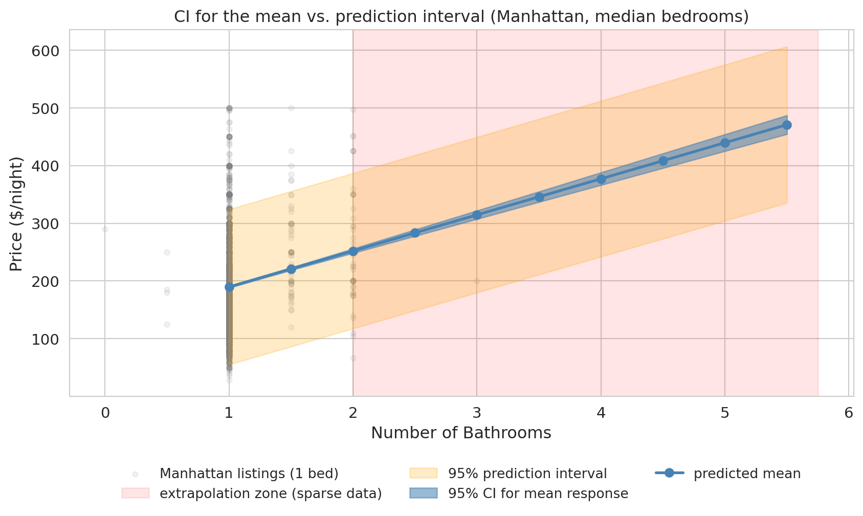
## Prediction intervals vs. confidence intervals
We have built confidence intervals for **coefficients** -- but what about predictions? When we use a regression model to predict at a particular value of $x$, there are two different questions, and they give different intervals.
- **Confidence interval for the mean response**: How uncertain are we about the *average* $Y$ at this $x$? This interval reflects estimation uncertainty in $\hat{\beta}$.
- **Prediction interval for a new observation**: Where might a *single new* $Y$ fall? This interval adds individual variability ($\varepsilon$) on top of estimation uncertainty.
:::{.callout-important}
## Prediction intervals are always wider
A **prediction interval** accounts for **two sources of uncertainty**: (1) estimation uncertainty in the regression line ($\hat{\beta}$ varies across hypothetical samples), and (2) individual variability around the line ($\varepsilon$ varies across listings). A confidence interval for the mean includes only source (1). The prediction interval is therefore always wider, and the gap grows with the residual variance: noisy responses produce much wider PIs than tight ones.
:::
:::{.callout-note collapse="true"}
## Going deeper: the half-width formulas
With the linear-algebra notation from Chapter 4, the prediction-interval half-width at a new point $x_0$ is $t^* \hat{\sigma} \sqrt{1 + x_0^\top (X^\top X)^{-1} x_0}$, where $\hat{\sigma}$ is the residual standard deviation. The CI half-width for the mean response drops the leading $1$ inside the square root. The leading $1$ is the contribution of individual variability ($\sigma^2$); the $x_0^\top (X^\top X)^{-1} x_0$ term is the estimation uncertainty in $\hat{\beta}$ at $x_0$.
:::
```{python}
# Prediction interval vs confidence interval — Airbnb model
bath_vals = np.arange(1, airbnb_clean['bathrooms'].max() + 0.5, 0.5)
grid = pd.DataFrame({
    'bathrooms': bath_vals,
    'bedrooms': [airbnb_clean['bedrooms'].median()] * len(bath_vals),
    'borough': ['Manhattan'] * len(bath_vals),
})
grid_pred = airbnb_model.get_prediction(grid).summary_frame(alpha=0.05)

fig, ax = plt.subplots(figsize=(9, 5.5))

# Underlying scatter: actual Manhattan listings at the median bedroom count.
median_beds = airbnb_clean['bedrooms'].median()
manhattan_data = airbnb_clean[
    (airbnb_clean['borough'] == 'Manhattan') &
    (airbnb_clean['bedrooms'] == median_beds)
]
ax.scatter(manhattan_data['bathrooms'], manhattan_data['price_clean'],
           alpha=0.10, s=14, color='gray', label=f'Manhattan listings ({int(median_beds)} bed)')

# Mark the extrapolation zone first so it sits behind the bands
data_max_bath = manhattan_data['bathrooms'].quantile(0.99)
ax.axvspan(data_max_bath, bath_vals.max() + 0.25, alpha=0.10, color='red',
           label='extrapolation zone (sparse data)')

ax.fill_between(bath_vals, grid_pred['obs_ci_lower'], grid_pred['obs_ci_upper'],
                alpha=0.22, color='orange', label='95% prediction interval')
ax.fill_between(bath_vals, grid_pred['mean_ci_lower'], grid_pred['mean_ci_upper'],
                alpha=0.55, color='steelblue', label='95% CI for mean response')
ax.plot(bath_vals, grid_pred['mean'], 'o-', color='steelblue',
        markersize=6, linewidth=2, label='predicted mean')

ax.set_xlabel('Number of Bathrooms', fontsize=12)
ax.set_ylabel('Price ($/night)', fontsize=12)
ax.set_title('CI for the mean vs. prediction interval (Manhattan, median bedrooms)',
             fontsize=12)
ax.tick_params(labelsize=11)

# Move legend below the plot so the bands have room
ax.legend(loc='upper center', bbox_to_anchor=(0.5, -0.16),
          ncol=3, fontsize=10, frameon=False)
plt.tight_layout()
plt.show()

print("The blue band (CI for the mean) is narrow — we are fairly sure about the average price.")
print("The orange band (prediction interval) is wide. Where the gray scatter is dense")
print("(near 1 bathroom), the band brackets most of it — exactly the job of a 95% PI.")
print("At higher bathroom counts, the band is extrapolated: few Manhattan-1-bedroom")
print("listings have 4-5 bathrooms, so we cannot visually verify coverage there.")
```
A specific prediction makes the difference concrete.
```{python}
# Numeric example: predicted price for a 2-bathroom, 2-bedroom Manhattan listing
example = pd.DataFrame({
    'bathrooms': [2],
    'bedrooms': [2],
    'borough': ['Manhattan'],
})
example_pred = airbnb_model.get_prediction(example).summary_frame(alpha=0.05)

print("Prediction for a 2-bath, 2-bed Manhattan listing:")
print(f"  Predicted price:        ${example_pred['mean'].values[0]:.2f}/night")
print(f"  95% CI for mean price:  [${example_pred['mean_ci_lower'].values[0]:.2f}, ${example_pred['mean_ci_upper'].values[0]:.2f}]")
print(f"  95% prediction interval:[${example_pred['obs_ci_lower'].values[0]:.2f}, ${example_pred['obs_ci_upper'].values[0]:.2f}]")
print()
print("The CI says the *average* listing like this rents for roughly")
print(f"${example_pred['mean_ci_lower'].values[0]:.0f}-${example_pred['mean_ci_upper'].values[0]:.0f}/night.")
print("The PI says a *single new* listing could fall anywhere in a much wider range,")
print("reflecting the large variation among individual Airbnb listings.")
```
## Q1 says yes — but is the effect big enough? (NBA cautionary tale)
The Airbnb story was tidy: the bathrooms coefficient is large, statistically distinguishable from zero, and stable enough to drive a renovation decision. Regression inference is not always so encouraging. We now turn the same machinery on a different question -- and watch the same machinery flag trouble.
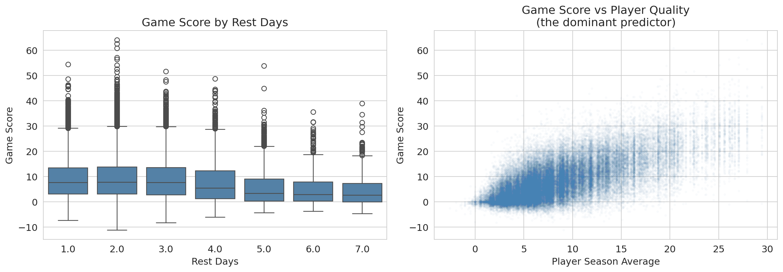
An NBA team's analytics department says rest boosts performance by about 0.3 game-score points per game -- enough to think about restructuring the schedule around it. Should the front office invest in roster flexibility based on that finding? Players who get more rest aren't a random subset of the league: coaches give bench players DNPs (extra rest by another name), they rest stars before tough matchups, and injured players return from long absences with high rest values. So a raw association between rest days and game score is tangled up with **who** is resting, on top of whatever rest itself does.
```{python}
# Load NBA data
nba = pd.read_csv(f'{DATA_DIR}/nba/nba_load_management.csv')
nba['GAME_DATE'] = pd.to_datetime(nba['GAME_DATE'])

# Drop rows missing REST_DAYS (a player's first game of the season has no prior rest);
# cap rest days at 7 to avoid treating long injury absences as "rest."
n_raw = len(nba)
nba_games = nba.dropna(subset=['REST_DAYS']).copy()
nba_games = nba_games[nba_games['REST_DAYS'] <= 7].copy()
print(f"NBA rows: {n_raw:,} raw, {len(nba_games):,} after dropping missing REST_DAYS and capping at 7 days")

# Compute player-season averages as a measure of player quality
nba_games['PLAYER_SEASON_AVG'] = nba_games.groupby(
    ['PLAYER_ID', 'SEASON']
)['GAME_SCORE'].transform('mean')

# Compute opponent game-score allowed (mean GAME_SCORE players post against this opponent)
# Note: HIGH value = opponent has a porous defense; LOW value = stingy defense.
opp_gs_allowed = nba_games.groupby('OPPONENT')['GAME_SCORE'].mean()
nba_games['OPP_GS_ALLOWED'] = nba_games['OPPONENT'].map(opp_gs_allowed)

# Derive additional covariates from existing columns
# Back-to-back indicator: did the player play yesterday?
nba_games['BACK_TO_BACK'] = (nba_games['REST_DAYS'] == 1).astype(int)

# Minutes in previous game (proxy for fatigue/usage)
nba_games = nba_games.sort_values(['PLAYER_ID', 'GAME_DATE'])
nba_games['PREV_MIN'] = nba_games.groupby('PLAYER_ID')['MIN'].shift(1)

print(f"Observations: {len(nba_games):,}")
print(f"Players: {nba_games['PLAYER_NAME'].nunique()}")
print()
print("Variables for regression:")
print(f"  GAME_SCORE (response): mean={nba_games['GAME_SCORE'].mean():.2f}, std={nba_games['GAME_SCORE'].std():.2f}")
print(f"  REST_DAYS: mean={nba_games['REST_DAYS'].mean():.2f}")
print(f"  PLAYER_SEASON_AVG: mean={nba_games['PLAYER_SEASON_AVG'].mean():.2f}")
print(f"  HOME: {nba_games['HOME'].mean():.2%} home games")
print(f"  OPP_GS_ALLOWED: mean={nba_games['OPP_GS_ALLOWED'].mean():.2f} (opponent's avg GS allowed; HIGH = porous defense)")
print(f"  BACK_TO_BACK: {nba_games['BACK_TO_BACK'].mean():.2%} of games")
print(f"  PREV_MIN: mean={nba_games['PREV_MIN'].mean():.1f} (previous game minutes)")
```
### Fit, then read
We predict `GAME_SCORE` from `REST_DAYS` plus three controls -- player season average, home/away, and the porousness of the opposing defense (`OPP_GS_ALLOWED`, the mean game score players post against that opponent; high = porous defense).
```{python}
model_full = smf.ols(
    'GAME_SCORE ~ REST_DAYS + PLAYER_SEASON_AVG + HOME + OPP_GS_ALLOWED',
    data=nba_games
).fit()

print(model_full.summary())
```
Read this table off the same template as Airbnb. The `REST_DAYS` row jumps out: coefficient $-0.15$, $p<0.001$, CI $[-0.20, -0.11]$ excludes zero comfortably. By the **Q1** criterion of block 1 -- "is the coefficient distinguishable from zero?" -- we have a winner.
**That is the surprise of the chapter.** Block 1 said a tight CI excluding zero meant decision-grade. Here, taking that seriously would say "rest hurts performance, $p<0.001$ -- cut rest days." That conclusion is wrong, and the next two questions tell us why.
:::{.callout-warning}
## Variable names can deceive
The `OPP_GS_ALLOWED` coefficient sits near $+1$, which looks paradoxical -- shouldn't a "stronger opponent" *lower* a player's score? Read the variable definition carefully: `OPP_GS_ALLOWED` is the average game score *allowed* by that opponent. High = porous defense. So a positive coefficient is mechanical: facing a porous defense → higher game score. The variable's name (had we called it `OPP_STRENGTH`) would have lied about the direction.
When a coefficient sign surprises you, before you write up "regression confirms X," look at how the variable was *constructed*. The most common source of a "surprising" sign is not a deep finding -- it is a sign convention you missed. The same lens applies to a coefficient that surprises in the *opposite* direction: a binary indicator coded `1 = no` rather than `1 = yes` flips the sign with no change in the underlying relationship.
:::
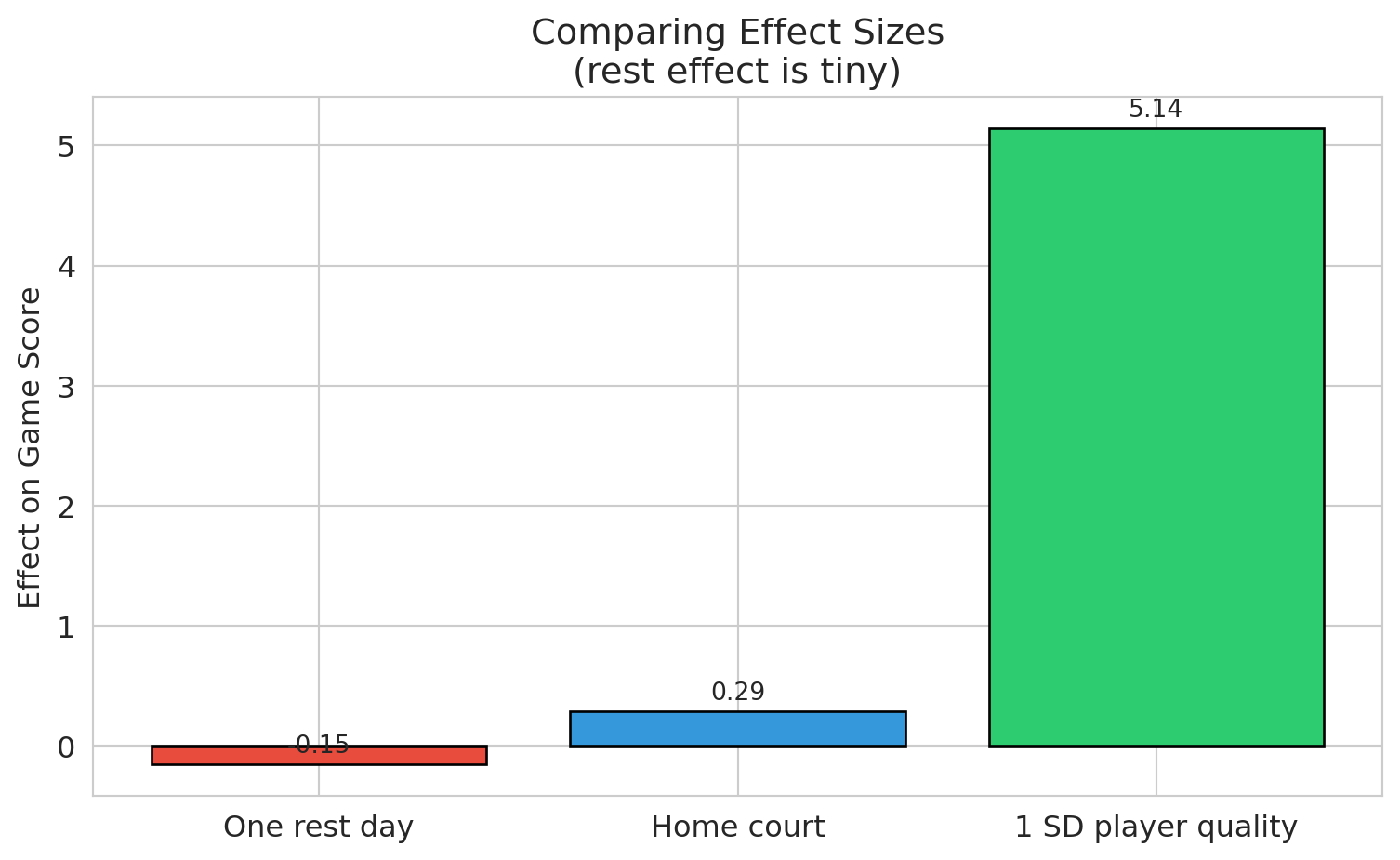
### Q2: is the effect large enough to matter?
Raw coefficients are hard to compare across predictors with different units. **Standardized coefficients** multiply each coefficient by its predictor's standard deviation, putting all effects on a common scale: "the effect of a one-SD change."
```{python}
# Two-panel: full scale (left) reveals player-quality dominance;
# zoomed (right) makes the small bars and their CIs readable.
ci = model_full.conf_int().drop('Intercept')
coef_vals = model_full.params.drop('Intercept')

predictor_sds = nba_games[['REST_DAYS', 'PLAYER_SEASON_AVG', 'HOME', 'OPP_GS_ALLOWED']].std()
std_coefs = coef_vals * predictor_sds
std_ci_lower = ci[0] * predictor_sds
std_ci_upper = ci[1] * predictor_sds

labels = ['Rest days', 'Player quality\n(season avg)', 'Home court', 'Opponent\nGS allowed']
y_pos = list(range(len(labels)))

# Color the bar that drives the decision differently so it pops in both panels.
colors = ['#e74c3c' if l == 'Rest days' else 'steelblue' for l in labels]

fig, axes = plt.subplots(1, 2, figsize=(10, 4.5),
                          gridspec_kw={'width_ratios': [1.4, 1]})

for ax, title, xlim in zip(
    axes,
    ['Full scale: player quality dominates',
     'Zoomed in: rest is essentially zero'],
    [None, (-0.5, 0.6)],
):
    ax.barh(y_pos, std_coefs.values, xerr=[
        std_coefs.values - std_ci_lower.values,
        std_ci_upper.values - std_coefs.values
    ], color=colors, edgecolor='black', capsize=5, alpha=0.75)
    ax.axvline(x=0, color='red', linestyle='--', linewidth=1)
    ax.set_yticks(y_pos)
    ax.set_yticklabels(labels)
    ax.set_xlabel('Effect of 1 SD change (game-score points)')
    ax.set_title(title, fontsize=11)
    if xlim is not None:
        ax.set_xlim(*xlim)

fig.suptitle('Standardized regression coefficients with 95% CIs', fontsize=12, y=1.02)
plt.tight_layout()
plt.show()

print("Left: player quality dwarfs everything else.")
print("Right: rest_days CI is fully visible — and it barely clears zero.")
```
The bar that should drive a strategic decision is a sliver next to the bars for the variables we already understood. With $n = 70{,}000$, the coefficient t-test is sensitive enough to flag effects too small to act on. The distinction has two formal names worth introducing:
- **Statistical significance**: the coefficient is distinguishable from zero given the sample (a property of the t-test, not the world).
- **Practical significance** (or **practical importance**): the coefficient is large enough to matter for a decision in the relevant domain (a property of the world, not the test).
To put effect sizes on a unitless scale comparable across problems, we use **Cohen's d** -- the coefficient divided by the response variable's standard deviation. The number you get is "how many SDs of the outcome does a one-unit change in the predictor move the prediction." Whether a given $d$ is "important" depends entirely on context: a tiny $d$ on something high-stakes (mortality, election margins) can matter; a "large" $d$ on something low-stakes can fail to. The benchmarks below are a backstop, not a substitute for asking "does this number change a decision?"
```{python}
# Effect size for REST_DAYS in NBA model
rest_coef = model_full.params['REST_DAYS']
rest_se = model_full.bse['REST_DAYS']
game_score_std = nba_games['GAME_SCORE'].std()

# Cohen's d: coefficient divided by outcome SD
std_effect = rest_coef / game_score_std

print("=== NBA Rest Effect: Significance vs Importance ===")
print()
print(f"Coefficient: {rest_coef:.3f} game score points per rest day")
print(f"Standard deviation of game score: {game_score_std:.2f}")
print(f"Cohen's d (standardized effect): {std_effect:+.4f} SD")
print(f"p-value: {format_pvalue(model_full.pvalues['REST_DAYS'])}")
print()
print("Cohen's (1988) rough behavioral-science benchmarks (use cautiously, see prose):")
print("  Small effect:  d ~ 0.2")
print("  Medium effect: d ~ 0.5")
print("  Large effect:  d ~ 0.8")
print(f"  Our effect:    d = {std_effect:+.4f}  <-- essentially zero on any benchmark")
print()
print(f"With n = {len(nba_games):,} observations, we can detect effects that are")
print(f"completely negligible in practice.")
```
> *"Statistical significance is no substitute for practical importance."* -- the unwritten lesson behind every $n$ in the tens of thousands.
:::{.callout-tip}
## Think about it
A sports analytics team comes to you and says "we ran a regression and found a negative coefficient for rest days -- extra rest actually *hurts* performance, with $p < 0.001$!" Before you act on that, what questions should you ask? Sketch your answers before reading on.
:::
1. How big is the effect? (Tiny -- a fraction of a point, standardized effect near zero.)
2. Is there confounding? (Yes -- coaches strategically rest players before tough opponents.)
3. Does the model capture all relevant factors? (No -- schedule difficulty, travel, fatigue history, etc.)
4. Would this result hold out of sample? (Uncertain.)
Statistical significance with large samples can detect effects **too small to matter**.
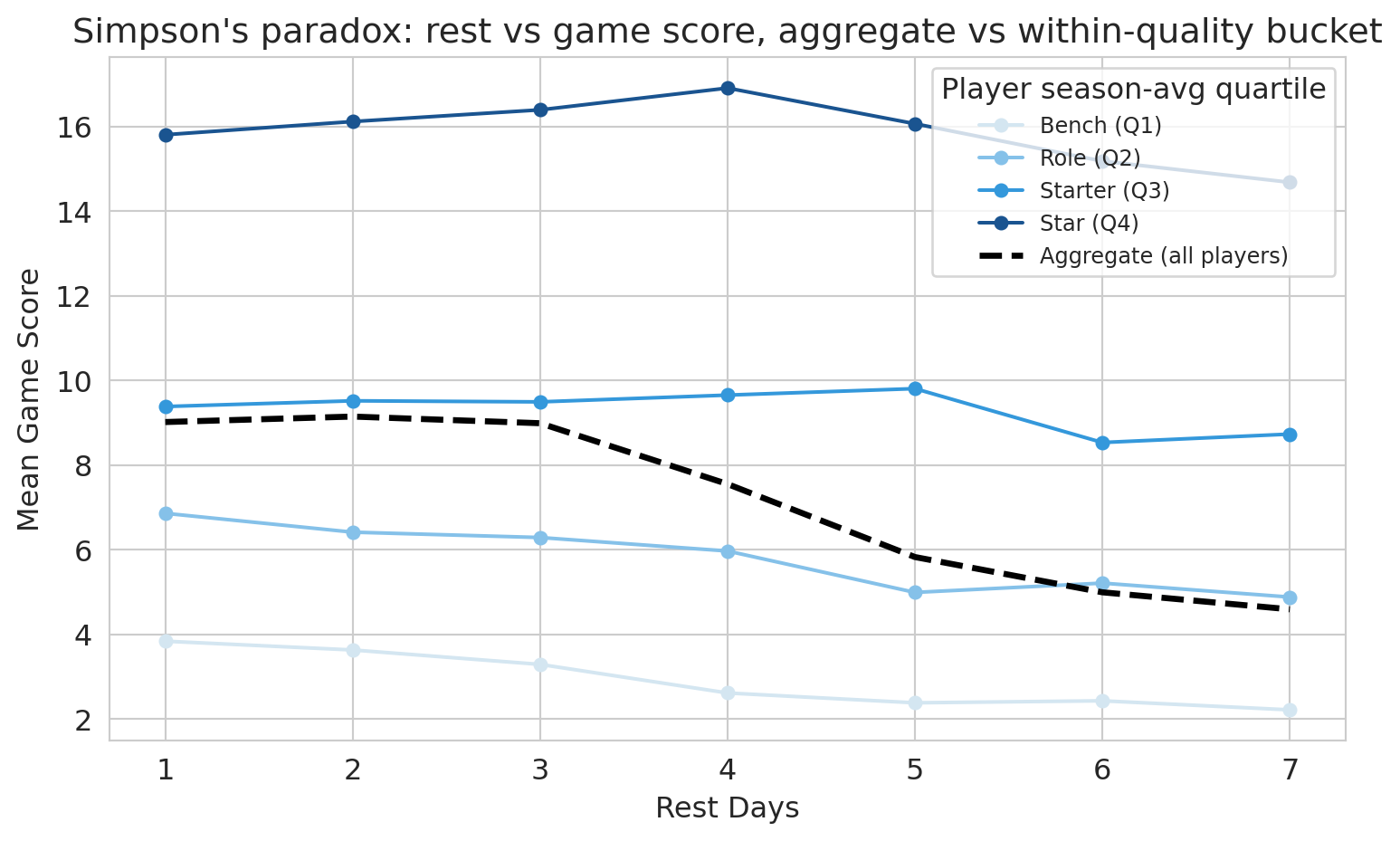
### Confounding made visible: aggregate vs. within-group slopes
The coefficient we just read controls for player quality. But the *naive* analysis -- regressing game score on rest days alone -- would have produced a different number entirely, and walking through why is a quick lesson in how confounding shapes what the regression reports.
The dashed line below shows the relationship between rest days and game score *aggregated across all players*. The colored lines show the same relationship *within* each player-quality quartile. If the aggregate slope and the within-bucket slopes disagree, the aggregate is a confounded estimate.
```{python}
# Simpson's paradox visualization: aggregate vs within-quality-bucket trend
nba_q = nba_games.copy()
nba_q['quality_bucket'] = pd.qcut(
    nba_q['PLAYER_SEASON_AVG'], q=4,
    labels=['Bench (Q1)', 'Role (Q2)', 'Starter (Q3)', 'Star (Q4)']
)

agg = nba_q.groupby('REST_DAYS', observed=True)['GAME_SCORE'].mean().reset_index()
buckets = (
    nba_q.groupby(['quality_bucket', 'REST_DAYS'], observed=True)['GAME_SCORE']
    .mean().reset_index()
)

fig, ax = plt.subplots(figsize=(8, 5))
for bucket, color in zip(['Bench (Q1)', 'Role (Q2)', 'Starter (Q3)', 'Star (Q4)'],
                         ['#d4e6f1', '#85c1e9', '#3498db', '#1a5490']):
    sub = buckets[buckets['quality_bucket'] == bucket]
    ax.plot(sub['REST_DAYS'], sub['GAME_SCORE'], 'o-',
            color=color, label=str(bucket), linewidth=1.5, markersize=5)
ax.plot(agg['REST_DAYS'], agg['GAME_SCORE'], 'k--',
        label='Aggregate (all players)', linewidth=2.5)
ax.set_xlabel('Rest days')
ax.set_ylabel('Mean game score')
ax.set_title("Simpson's paradox: rest vs game score, aggregate vs within-quality bucket")
ax.legend(title='Player season-avg quartile', fontsize=9, loc='best')
plt.tight_layout()
plt.show()
```
The four colored within-bucket lines are nearly flat: once we compare like-to-like, extra rest barely moves game score. The dashed aggregate line moves more, because it picks up the compositional effect of which players are at each rest value. Adding `PLAYER_SEASON_AVG` to the regression is the algebraic version of switching from the dashed line to the colored ones. This is **Simpson's paradox in regression form**: an aggregate association that flips or shrinks once we condition on the right covariate. Here the *signs* are the same -- aggregate and within-bucket slopes both trend slightly down -- but the aggregate is much steeper. So this example is the *attenuation* flavor of Simpson's, not a sign-flip; the lesson is the same either way: an unadjusted regression of game score on rest days alone would have reported a misleadingly large coefficient.
:::{.callout-warning}
## Association, not causation
Our regression controls for measured covariates -- player quality, home court, opponent porousness -- but it does NOT estimate a *causal* effect of rest. Coaches choose when to rest players for strategic reasons we cannot observe (a DNP after a soft loss differs from a DNP before a back-to-back). Chapter 18 introduces directed acyclic graphs (DAGs), the framework that lets you draw which paths a regression closes and which it leaves open -- and decide whether "controlling for" was enough.
:::
## Q3: is the inference trustworthy?
You met residual plots in Chapter 5 as a tool for spotting missing model structure (curves, clusters, fans). Here we use the same plots for a sharper purpose: deciding whether the t-tests and confidence intervals above can be trusted at all. We have run the same machinery on two regressions and gotten very different answers; before we trust either, we have to check that the formula-based inference rests on a sound foundation. The diagnostics below apply to BOTH models in turn.
:::{.callout-important}
## Definition: LINE Conditions
The assumptions for regression inference are remembered by the **LINE** mnemonic:
- **L**inearity: the relationship between predictors and response is linear.
- **I**ndependence: observations are independent of each other.
- **N**ormality: residuals are approximately normally distributed.
- **E**qual variance: the spread of residuals is roughly constant across fitted values (no **heteroscedasticity**).
:::
Each LINE condition has a characteristic diagnostic signature. The residual plot below addresses **L** (linearity, via the LOWESS curve) and **E** (equal variance, via the scale-location panel); the Q-Q plot addresses **N** (normality). The fourth letter, **I** (independence), is harder to check from residual plots alone -- it requires you to ask whether the rows are clustered. Both datasets here have an independence concern worth flagging: NBA observations are repeated player-game records (the same player appears thousands of times, so games for one player share unmeasured traits), and Airbnb listings cluster by host (one host with many listings shares pricing strategy and amenity quality). The standard fix is **clustered standard errors**, which inflate the SEs to reflect the within-cluster correlation. With sample sizes in the tens of thousands, clustering would widen the bathroom and rest-day CIs but would not flip a "significant vs not" conclusion or change which coefficients dominate -- the qualitative findings stand. We leave the implementation to homework, where you will also generate synthetic data that violates each LINE assumption and create the corresponding diagnostic plots.
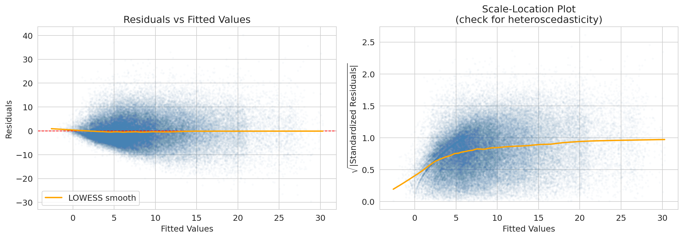
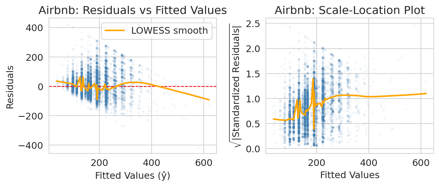
### Residual plot: do residuals have constant spread?
:::{.callout-important}
## Definition: Residual plot
A **residual plot** shows residuals (observed $-$ predicted) vs. **fitted values** (the model's predicted values, $\hat{y}_i$). We want to see a random scatter with no pattern. If the spread of residuals changes with the fitted value, that is **heteroscedasticity** -- the model's uncertainty is not uniform.
:::
The x-axis of the residual plot shows the **fitted values** -- the model's predicted response for each observation, $\hat{y}_i$. The orange curve is a **LOWESS smooth** (locally weighted scatterplot smoothing): a flexible local average that highlights any systematic trend. A flat LOWESS line near zero suggests the assumptions are met; a bend or funnel shape signals a problem.
```{python}
# Residual plot for the Airbnb model
fitted_air = airbnb_model.fittedvalues
resid_air = airbnb_model.resid

fig, axes = plt.subplots(1, 2, figsize=(8, 3.5))

axes[0].scatter(fitted_air, resid_air, alpha=0.04, s=5, color='steelblue')
axes[0].axhline(y=0, color='red', linestyle='--', linewidth=1)
axes[0].set_xlabel('Fitted values (ŷ)')
axes[0].set_ylabel('Residuals')
axes[0].set_title('Airbnb: residuals vs fitted values')
smooth_air = lowess(resid_air, fitted_air, frac=0.1)
axes[0].plot(smooth_air[:, 0], smooth_air[:, 1], color='orange', linewidth=2, label='LOWESS smooth')
axes[0].legend()

std_resid_air = airbnb_model.get_influence().resid_studentized_internal
axes[1].scatter(fitted_air, np.sqrt(np.abs(std_resid_air)), alpha=0.04, s=5, color='steelblue')
axes[1].set_xlabel('Fitted values')
axes[1].set_ylabel(r'$\sqrt{|\mathrm{Standardized\ Residuals}|}$')
axes[1].set_title('Airbnb: scale-location plot')
smooth_air2 = lowess(np.sqrt(np.abs(std_resid_air)), fitted_air, frac=0.1)
axes[1].plot(smooth_air2[:, 0], smooth_air2[:, 1], color='orange', linewidth=2)

plt.tight_layout()
plt.show()

print("Airbnb: spread of residuals fans out as fitted price grows — a textbook funnel.")
print("Expensive listings vary more in absolute dollars than cheap ones do, so the")
print("constant-variance assumption (the 'E' in LINE) is mildly violated. Options below.")
```
:::{.callout-note collapse="true"}
## Going deeper: NBA residual diagnostics
The NBA model has the same E-violation in a different form. The residuals look roughly symmetric around zero, but the scale-location LOWESS rises from ~0.2 at low fitted scores to ~1.0 at high ones — players projected to score low have less room to deviate; high-projection stars have wider game-to-game swings. The plotting code is parallel to the Airbnb diagnostic above; just substitute `model_full` for `airbnb_model`.
```python
fitted_nba = model_full.fittedvalues
resid_nba = model_full.resid
fig, axes = plt.subplots(1, 2, figsize=(8, 3.5))
axes[0].scatter(fitted_nba, resid_nba, alpha=0.02, s=5, color='steelblue')
axes[0].axhline(y=0, color='red', linestyle='--', linewidth=1)
# ... (same as Airbnb residual plot)
```
:::
### Q-Q plot: are residuals approximately normal?
A **Q-Q plot** compares residual quantiles to what we would expect from a normal distribution. Points on the diagonal indicate normality. Deviations in the tails indicate heavy tails or skew.
```{python}
# Q-Q plot for the Airbnb model
fig, ax = plt.subplots(figsize=(6, 6))
(tq_air, ord_air), (slope_air, intercept_air, _) = stats.probplot(resid_air, dist='norm')
ax.scatter(tq_air, ord_air, alpha=0.04, s=5, color='steelblue')
ref_x = np.array([tq_air.min(), tq_air.max()])
ax.plot(ref_x, intercept_air + slope_air * ref_x, 'r-', linewidth=1.5, label='Normal reference line')
ax.set_xlabel('Theoretical quantiles (normal)')
ax.set_ylabel('Sample quantiles (residuals)')
ax.set_title('Q-Q Plot of Residuals\n(Airbnb regression model)')
ax.legend()
plt.tight_layout()
plt.show()

print("Airbnb residuals are right-skewed: prices have a hard floor near $0 but a long")
print("right tail (a few listings far above the mean). The right tail of the Q-Q plot bows")
print("up; the left side tracks the line. Combined with the heteroscedasticity above, this")
print("suggests a log-price transformation would clean both problems up.")
```
:::{.callout-note collapse="true"}
## Going deeper: NBA Q-Q plot
The NBA Q-Q tells a milder version of the same right-skew story. Read it one tail at a time: the left tail is closer to the normal line than the right tail is, though not perfectly so (mild deviation in the moderate-negative range). The right tail bows above the line — the biggest games (a star going 12-for-15 from three) happen more often than a normal would allow. With $n > 70{,}000$ the CLT rescues formula-based inference on the coefficients; a *prediction interval* for an individual game score would be too narrow on the high end.
:::
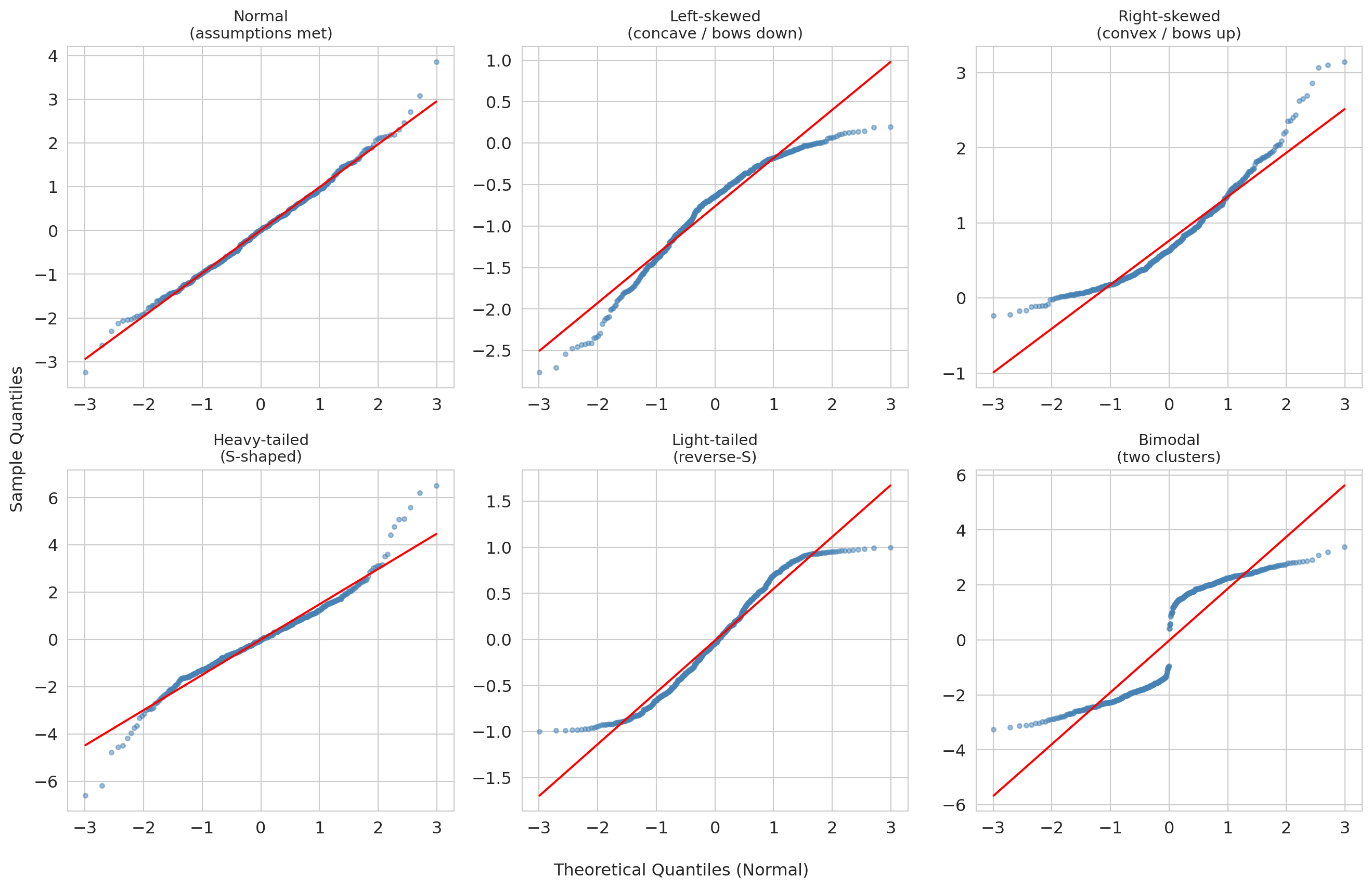
:::{.callout-note collapse="true"}
## Going deeper: Q-Q gallery — reading other departures from normality
Both Airbnb and NBA residuals showed right-skew (the right tail bows up while the left tail tracks the line). What do other departures from normality look like? The gallery below pairs each residual distribution (top row of each block) with its Q-Q plot (bottom row), so you can read directly from distribution shape to Q-Q shape.
```{python}
#| label: fig-qq-gallery
#| fig-cap: "Q-Q plot gallery: six residual distributions paired with their Q-Q plots. The top row of each block shows the distribution; the bottom row shows the corresponding Q-Q plot."
from scipy.stats import probplot, skewnorm, t as t_dist, uniform

np.random.seed(42)
n_sim = 500

# Simulate six residual distributions
sim_data = {
    'Normal\n(assumptions met)': np.random.normal(0, 1, n_sim),
    'Left-skewed\n(concave / bows down)': skewnorm.rvs(-8, size=n_sim),
    'Right-skewed\n(convex / bows up)': skewnorm.rvs(8, size=n_sim),
    'Heavy-tailed\n(S-shaped)': t_dist.rvs(df=3, size=n_sim),
    'Light-tailed\n(reverse-S)': uniform.rvs(loc=-1, scale=2, size=n_sim),
    'Bimodal\n(two clusters)': np.concatenate([
        np.random.normal(-2, 0.5, n_sim // 2),
        np.random.normal(2, 0.5, n_sim // 2)
    ]),
}

annotations = {
    'Normal\n(assumptions met)': None,
    'Left-skewed\n(concave / bows down)': {'text': 'left tail too\nspread out', 'xy_frac': (0.15, 0.10), 'arrow_frac': (0.12, 0.22)},
    'Right-skewed\n(convex / bows up)': {'text': 'right tail too\nspread out', 'xy_frac': (0.65, 0.85), 'arrow_frac': (0.88, 0.82)},
    'Heavy-tailed\n(S-shaped)': {'text': 'both tails\nheavier than normal', 'xy_frac': (0.55, 0.15), 'arrow_frac': (0.88, 0.08)},
    'Light-tailed\n(reverse-S)': {'text': 'both tails\nlighter than normal', 'xy_frac': (0.15, 0.75), 'arrow_frac': (0.12, 0.88)},
    'Bimodal\n(two clusters)': {'text': 'gap = two\nsubgroups', 'xy_frac': (0.35, 0.55), 'arrow_frac': (0.50, 0.50)},
}

# Lay out the six distributions in two blocks of three columns.
# Each block: top row = density, bottom row = Q-Q plot.
row_layouts = [
    ['Normal\n(assumptions met)', 'Left-skewed\n(concave / bows down)', 'Right-skewed\n(convex / bows up)'],
    ['Heavy-tailed\n(S-shaped)', 'Light-tailed\n(reverse-S)', 'Bimodal\n(two clusters)'],
]

fig, axes = plt.subplots(4, 3, figsize=(14, 12),
                         gridspec_kw={'height_ratios': [1, 1.4, 1, 1.4]})

for block_idx, labels in enumerate(row_layouts):
    density_row = block_idx * 2
    qq_row = block_idx * 2 + 1
    for col, label in enumerate(labels):
        data = sim_data[label]

        # Density (top of this block)
        ax_d = axes[density_row, col]
        ax_d.hist(data, bins=40, density=True, color='lightsteelblue', edgecolor='white')
        ax_d.set_title(label, fontsize=11)
        ax_d.set_yticks([])
        ax_d.set_xlabel('')
        if col == 0:
            ax_d.set_ylabel('density', fontsize=10)

        # Q-Q plot (bottom of this block)
        ax_q = axes[qq_row, col]
        (tq, sq), (slope, intercept, _) = probplot(data, dist='norm')
        ax_q.scatter(tq, sq, s=10, alpha=0.5, color='steelblue')
        ref_x = np.array([tq.min(), tq.max()])
        ax_q.plot(ref_x, intercept + slope * ref_x, 'r-', linewidth=1.5)
        if block_idx == len(row_layouts) - 1:
            ax_q.set_xlabel('Theoretical quantiles (normal)', fontsize=10)
        if col == 0:
            ax_q.set_ylabel('Sample quantiles', fontsize=10)

        # Annotation arrow linking the Q-Q shape to the failure mode
        ann = annotations.get(label)
        if ann is not None:
            xlim, ylim = ax_q.get_xlim(), ax_q.get_ylim()
            xy = (xlim[0] + ann['arrow_frac'][0] * (xlim[1] - xlim[0]),
                  ylim[0] + ann['arrow_frac'][1] * (ylim[1] - ylim[0]))
            xytext = (xlim[0] + ann['xy_frac'][0] * (xlim[1] - xlim[0]),
                      ylim[0] + ann['xy_frac'][1] * (ylim[1] - ylim[0]))
            ax_q.annotate(ann['text'], xy=xy, xytext=xytext, fontsize=8,
                          color='#e74c3c', fontweight='bold',
                          arrowprops=dict(arrowstyle='->', color='#e74c3c', lw=1.5),
                          ha='center', va='center')

plt.tight_layout()
plt.show()
```
**How to read the gallery:**
| Q-Q shape | What it means | Example cause |
|:--|:--|:--|
| Straight line | Normal residuals — assumptions satisfied | Well-specified model |
| Concave (bows down) | Left-skewed residuals | Floor effect or bounded response |
| Convex (bows up) | Right-skewed residuals | Untransformed prices or counts |
| S-shaped | Heavy tails — more extreme values than normal | Outlier-prone measurements |
| Reverse-S | Light tails — fewer extreme values than normal | Bounded or truncated data |
| Staircase or gap | Multimodal residuals — distinct subgroups | Missing categorical predictor |
The key diagnostic reflex: when the Q-Q plot bows or bends, ask *why* the residuals deviate from normality. The shape often points directly to a modeling fix (a log transform, a missing predictor, or an outlier filter).
:::
A note on why we look at residuals rather than the raw response: residuals remove the variation explained by the other predictors, so a pattern (curvature, fan, cluster) that was invisible in the raw $y$-vs-$x$ scatter often jumps out in the residual plot.
:::{.callout-warning}
## When diagnostics reveal problems
If residuals show strong non-normality or heteroscedasticity, the formula-based standard errors and p-values may be unreliable. Options include:
- **Bootstrap confidence intervals** (Chapter 8) do not assume normality -- they let the data speak for itself.
- **Robust standard errors** (standard errors adjusted to remain valid even when the residual variance is not constant across observations) protect your inference against heteroscedasticity without changing the coefficient estimates.
- **Transform the response** (e.g., log price) to stabilize variance.
:::
For both models in this chapter, the sample sizes are large ($n \approx 15{,}000$ for Airbnb, $n \approx 72{,}000$ for NBA), so the CLT still buys us approximately correct formula-based inference on the coefficients despite the right-skewed residuals. With smaller samples or heavier tails, bootstrap CIs would be the safer choice -- and our bootstrap on the bathrooms coefficient already agreed with the formula, which is itself a useful sanity check.
:::{.callout-warning}
## Diagnostics catch statistical problems, not systematic ones
Residual plots, Q-Q plots, and the LINE conditions catch *statistical* problems: non-normality, heteroscedasticity, the wrong functional form. They do *not* catch the *systematic* problems that make a regression coefficient a biased answer to a causal question -- selective treatment assignment, omitted variables, model misspecification you have not thought to check. The NBA REST_DAYS coefficient is the canonical case in point: with $n > 70{,}000$ its CI is statistically tight, and the diagnostic plots above are mostly clean. Yet the coefficient would still be the wrong answer to "should we rest players more?" if rested players were also strategically scheduled against weaker opponents -- a confounder regression cannot adjust for unless we measure it. **Confidence intervals widen with sample noise; they do not widen with confounding.**
:::
## Putting it together: Airbnb vs NBA
Both analyses used the same tools -- t-tests and confidence intervals on regression coefficients. The conclusions differ dramatically.
```{python}
# Side-by-side comparison
print("=" * 60)
print(f"{'':30s} {'Airbnb Bath':>12s}  {'NBA Rest':>12s}")
print("=" * 60)
print(f"{'Coefficient':30s} {beta_bath:12.2f}  {rest_coef:12.3f}")
print(f"{'SE':30s} {se_bath:12.4f}  {rest_se:12.4f}")
print(f"{'p-value':30s} {format_pvalue(p_bath):>12s}  {format_pvalue(model_full.pvalues['REST_DAYS']):>12s}")
ci_rest = model_full.conf_int().loc['REST_DAYS']
print(f"{'95% CI lower':30s} {ci_bath[0]:12.2f}  {ci_rest[0]:12.3f}")
print(f"{'95% CI upper':30s} {ci_bath[1]:12.2f}  {ci_rest[1]:12.3f}")
std_effect_label = "Standardized effect (coef/SD)"
print(f"{std_effect_label:30s} {beta_bath/airbnb_clean['price_clean'].std():12.4f}  {std_effect:12.4f}")
print(f"{'n':30s} {int(airbnb_model.nobs):12,d}  {len(nba_games):12,d}")
print(f"{'Practically meaningful?':30s} {'Yes':>12s}  {'No':>12s}")
print("=" * 60)
print()
print("Both are 'statistically significant.' Only one is large enough to act on.")
```
## Inference for logistic regression
Chapter 7 introduced logistic regression: coefficients live on the log-odds scale, and $e^{\hat{\beta}_j}$ is the **odds ratio** — the multiplicative change in odds per unit increase in $x_j$.
If you have ever looked at sports betting lines, you already have intuition for odds ratios. A betting line of "+200" on Stanford football means a winning \$1 bet pays \$2, implying the bookmaker's odds against Stanford are 2-to-1, or odds of 1/3 on Stanford winning. If a coaching change moves the line from +200 to +100 (1-to-1), the odds against Stanford have *halved* — an odds ratio of $1/2$. The OR is the multiplicative shift in betting odds you would see on the board. Logistic regression is the same accounting, computed from data: each $e^{\hat\beta_j}$ tells you how much the odds of the outcome change when $x_j$ moves by one unit, holding everything else fixed.
The same inference machinery from linear regression applies to the $\hat{\beta}_j$: standard errors, test statistics, p-values, and confidence intervals. Only two things change:
- The test statistic is labeled **z** instead of **t**, because logistic regression uses the **Wald test**: a maximum-likelihood-based statistic that is *asymptotically normal* by general MLE theory. There is no exact small-sample distribution analogous to the OLS $t_{n-p-1}$, so software always returns a $z$ and a normal-based p-value -- accurate at the sample sizes you will encounter in this course, less reliable for rare-event outcomes or near-perfect separation.
- A 95% CI $[a, b]$ on $\hat{\beta}_j$ exponentiates directly to a 95% CI $[e^a, e^b]$ on the odds ratio (the exponential function is monotone).
We return to the **Framingham Heart Study** from Chapter 7, this time with a smaller model of six clinically meaningful predictors. To match Chapter 7's setup, we standardize the features — so coefficients and odds ratios are interpreted per one-SD change in each predictor.
```{python}
# Load Framingham data and drop rows with missing values
framingham = pd.read_csv(f'{DATA_DIR}/framingham/framingham.csv')
fram = framingham.dropna().copy()
print(f"Complete cases: {len(fram):,} of {len(framingham):,}")
```
We fit on standardized features so each coefficient -- and each odds ratio -- has the same "per one-SD change in this predictor" interpretation.
```{python}
# Fit logistic regression with statsmodels on standardized features
y = fram['TenYearCHD']
feature_cols = ['age', 'male', 'BMI', 'sysBP', 'cigsPerDay', 'glucose']
X_raw = fram[feature_cols]
X = (X_raw - X_raw.mean()) / X_raw.std()  # standardize
X = sm.add_constant(X)

logit_model = sm.Logit(y, X).fit(disp=0)
print(logit_model.summary())
```
The table reads off the same template as the OLS outputs above, with z-statistics in place of t-statistics.
### Odds ratios and confidence intervals
Exponentiate the fitted coefficients and their CIs to get odds ratios with CIs.
```{python}
# Compute odds ratios with 95% CIs
ci = logit_model.conf_int()
coef_table = pd.DataFrame({
    'Odds Ratio': np.exp(logit_model.params),
    'OR 95% CI Lower': np.exp(ci[0]),
    'OR 95% CI Upper': np.exp(ci[1]),
    'p-value': logit_model.pvalues,
})

# Display without the intercept (odds ratio for the intercept is not meaningful)
print(coef_table.loc[coef_table.index != 'const'].round(4).to_string())
```
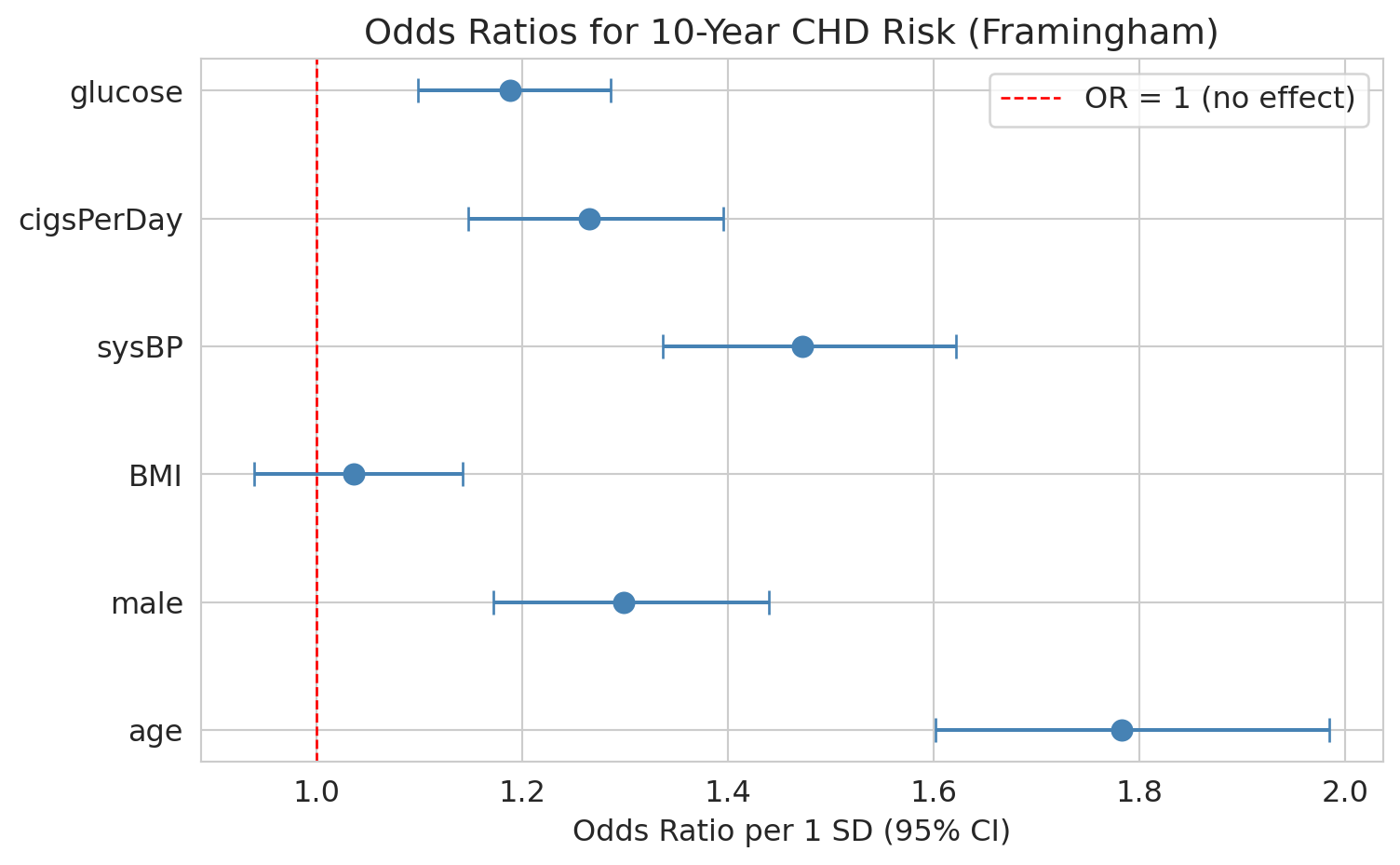
Because the features are standardized, each odds ratio is the multiplicative change in odds per **one-SD** increase in that predictor, holding the others constant.
Walk through `age` concretely. Its standardized OR is roughly 1.7, so each one-SD increase in age (about 9 years in this cohort) multiplies the odds of 10-year CHD by 1.7 -- about a 70% increase. Going from age 50 to 60 is a bit more than one SD, so the odds multiply by roughly $1.7 \times 1.7^{1/9} \approx 1.85$. To get a per-year odds ratio directly, divide the coefficient by the feature's SD before exponentiating: $\exp(\hat\beta_{\text{age}} / \mathrm{SD}_{\text{age}})$. The forest plot below shows all six ORs side by side.
```{python}
#| code-fold: true
# Forest plot of odds ratios
predictors = [p for p in logit_model.params.index if p != 'const']
ors = np.exp(logit_model.params[predictors])
or_ci_lower = np.exp(ci.loc[predictors, 0])
or_ci_upper = np.exp(ci.loc[predictors, 1])

fig, ax = plt.subplots(figsize=(8, 5))
y_pos = range(len(predictors))
ax.errorbar(ors, y_pos, xerr=[ors - or_ci_lower, or_ci_upper - ors],
            fmt='o', color='steelblue', capsize=5, markersize=8)
ax.axvline(x=1, color='red', linestyle='--', linewidth=1, label='OR = 1 (no effect)')
ax.set_yticks(list(y_pos))
ax.set_yticklabels(predictors)
ax.set_xlabel('Odds ratio per 1 SD (95% CI)')
ax.set_title('Odds ratios for 10-year CHD risk (Framingham)')
ax.legend()
plt.tight_layout()
plt.show()
```
An odds ratio whose CI excludes 1 is statistically significant; one whose CI includes 1 is not distinguishable from "no effect."
**Next up:** [Chapter 12.5](lec12.5-classification-inference.qmd) takes the same machinery to classification: bootstrap CIs for AUC, permutation tests for whether a classifier beats random guessing, and multiple-testing corrections over many logistic coefficients. Both chapters share the same template -- only the test statistic and the response variable change. Then [Chapter 13](lec13-trees.qmd) opens Act 3 with a completely different model family: decision trees and random forests.
## Key takeaways
1. **Regression inference asks: is each predictor useful in this model?** The **coefficient t-test** tests $H_0: \beta_j = 0$ — given the other predictors. The null is conditional, not absolute.
2. **Read every regression table off the same template:** coef, SE, t, p, CI, $R^2$, F, condition number. Variable names can lie about the encoding -- always interpret signs in light of how the variable was *constructed*.
3. **Confidence intervals tell you the range of plausible effect sizes.** A wide CI signals imprecision; a CI that barely excludes zero should make you cautious.
4. **Statistical significance $\neq$ practical importance.** With large $n$, the t-test can flag effects too small to act on. Always report effect sizes alongside p-values.
5. **Context determines whether a result is actionable.** The bathroom premium (about \$60/night) clears a renovation hurdle. The rest effect (a fraction of a game-score point) does not justify restructuring an NBA schedule.
6. **Diagnostics decide whether the inference is trustworthy.** Residual plots flag heteroscedasticity (Airbnb prices fan out at the high end); Q-Q plots flag non-normality (both models showed right-skew). Large $n$ rescues coefficient inference via the CLT, but prediction intervals still rely on the residual distribution.
7. **Regression estimates associations, not causal effects.** Both regressions adjust for measured covariates, but neither establishes causation. We return to this distinction in Chapter 18.
## Study guide
### Key ideas
- **Coefficient t-test**: Tests whether a single regression coefficient is significantly different from zero, conditional on the other predictors. $t = \hat{\beta}_j / \widehat{\text{SE}}(\hat{\beta}_j)$.
- **Standard error (of a coefficient)**: The estimated standard deviation of $\hat{\beta}_j$ across repeated samples. Measures uncertainty in the coefficient estimate.
- **Conditional null hypothesis**: $\beta_j = 0$ given the other predictors in the model. The same predictor can pass in one model and fail in another.
- **Controlling for** / **holding constant**: The regression interpretation -- the effect of one predictor after accounting for the others in the model.
- **Practical significance**: Whether an effect is large enough to matter in context, regardless of the p-value.
- **Effect size**: A standardized measure of how large an effect is (e.g., coefficient divided by the outcome's SD).
- **Residual plot**: Scatter plot of residuals vs. fitted values; used to check for patterns, non-linearity, and heteroscedasticity.
- **Q-Q plot**: Quantile-quantile plot comparing residual quantiles to a normal distribution; points on the diagonal indicate normality.
- **Heteroscedasticity**: When the variance of residuals changes across fitted values (the spread "fans out"). Violates the constant-variance assumption of OLS inference.
- **LINE conditions**: The four assumptions for regression inference -- Linearity, Independence, Normality, Equal variance.
- **Prediction interval**: An interval for where a *single new* observation might fall at a given $x$. Always wider than the confidence interval for the mean -- it includes both estimation uncertainty and individual variability.
- **Parsimony / Occam's razor**: The best model is the simplest one that adequately fits the data. Drop predictors that are not useful.
- **Wald test** (for logistic regression coefficients): asymptotically-normal analog of the t-test; the z-statistic $\hat{\beta}_j / \widehat{\text{SE}}(\hat{\beta}_j)$ is compared to a standard normal. CIs on $\hat{\beta}_j$ map to CIs on the odds ratio $e^{\hat{\beta}_j}$ by exponentiating.
### Computational tools
- `smf.ols('y ~ x1 + x2', data=df).fit()` -- fit an OLS regression with formula syntax
- `model.summary()` -- full regression output including coefficients, SEs, t-stats, p-values
- `model.params` -- dictionary of fitted coefficients
- `model.pvalues` -- dictionary of p-values for each coefficient's t-test
- `model.conf_int()` -- 95% confidence intervals for all coefficients
- `model.bse` -- standard errors of all coefficients
- `model.fittedvalues`, `model.resid` -- fitted values and residuals for diagnostic plots
- `model.get_prediction(new_data).summary_frame()` -- confidence interval for the mean and prediction interval for a new observation
- `stats.probplot(residuals, dist='norm')` -- Q-Q plot data with correct scaling
- `format_pvalue(p)` -- format p-values in scientific notation when below 0.001
- `sm.Logit(y, X).fit().summary()` -- fit logistic regression with inference (coefficients, SEs, z-statistics, p-values, CIs)
### For the quiz
- Be able to interpret a full regression output table: read off coefficients, standard errors, t-statistics, p-values, R-squared, F-statistic, and condition number.
- Know what "controlling for" means in a regression context and how the conditional null shapes the t-test.
- Distinguish statistical significance (small p-value) from practical importance (large effect size).
- Know the formula $t = \hat{\beta}_j / \widehat{\text{SE}}(\hat{\beta}_j)$ and what it tests.
- Be able to interpret a confidence interval for a regression coefficient in context.
- Know what a residual plot and Q-Q plot show, and what patterns indicate problems (heteroscedasticity, non-normality).
- Know the LINE conditions (Linearity, Independence, Normality, Equal variance) and which diagnostic plots check which conditions.
- Know that bootstrap CIs (Chapter 8) are a fallback when normality assumptions fail.
- Be able to interpret a logistic regression inference table: read off z-statistics, p-values, and CIs, and convert coefficients and CIs to odds ratios.