Decision Trees and Random Forests

Download notebook (.ipynb)

You’re building a pricing tool for Airbnb hosts and your manager wants a working prototype by Friday. Feature engineering (Chapter 5) got you a reasonable R² — but you had to pick which interactions to include, which polynomial degree, and how to encode dozens of neighborhoods. Do you spend the week hand-engineering features, or is there a model that figures out where to split on its own?

Decision trees do exactly that: they find the splits automatically. No encoding, no polynomial terms, no missing-value imputation. Today: how a tree splits, why a single tree overfits, how a forest fixes that by averaging, and when (despite all that) you should still reach for logistic regression instead.

Two model families × two tasks

	Regression	Classification
Linear models	Linear regression (Ch 4–5)	Logistic regression (Ch 7)
Trees	Regression tree (today)	Classification tree (today)

For trees, regression and classification differ only in the splitting criterion.

Code

import numpy as np
import pandas as pd
import matplotlib.pyplot as plt
import seaborn as sns
from sklearn.tree import DecisionTreeRegressor, DecisionTreeClassifier, plot_tree, export_text
from sklearn.ensemble import RandomForestRegressor, RandomForestClassifier
from sklearn.linear_model import LinearRegression, LogisticRegression
from sklearn.model_selection import train_test_split, cross_val_score
from sklearn.metrics import (r2_score, confusion_matrix,
                             precision_score, recall_score, f1_score,
                             roc_curve, roc_auc_score, ConfusionMatrixDisplay)
import warnings
warnings.filterwarnings('ignore')
sns.set_style('whitegrid')
plt.rcParams['figure.figsize'] = (8, 5)
plt.rcParams['font.size'] = 12

The data: Airbnb NYC listings

Code

DATA_DIR = 'data'
listings = pd.read_csv(f'{DATA_DIR}/airbnb/listings.csv', low_memory=False)

cols = ['id', 'name', 'description', 'price', 'bedrooms', 'bathrooms', 'room_type',
        'neighbourhood_group_cleansed', 'accommodates', 'number_of_reviews',
        'latitude', 'longitude']
df = listings[cols].dropna(subset=['price', 'bedrooms', 'bathrooms']).copy()
df = df.rename(columns={'neighbourhood_group_cleansed': 'borough'})
df['price'] = pd.to_numeric(df['price'].astype(str).str.replace('[$,]', '', regex=True), errors='coerce')
df = df[df['price'].between(10, 500)].reset_index(drop=True)
prices = df['price']

print(f"Working with {len(df):,} listings")
df[['name', 'price', 'bedrooms', 'bathrooms', 'room_type', 'borough']].head()

Working with 28,778 listings

	name	price	bedrooms	bathrooms	room_type	borough
0	Cozy Stay in Queens, Easy Access to Manhattan	45	1	1.0	Private room	Queens
1	Spacious room in comfortable apt.	95	1	1.0	Private room	Manhattan
2	Fresh Clean & Modern: Williamsburg at its Best	60	1	1.5	Entire home/apt	Brooklyn
3	Cozy Room In Perfect Location!	70	1	1.0	Private room	Manhattan
4	Charming Central Park Studio	104	1	1.0	Entire home/apt	Manhattan

Same feature matrix as Chapter 5: numeric features plus one-hot encoded categoricals.

Code

cat_features = pd.get_dummies(df[['room_type', 'borough']], drop_first=True)
num_features = df[['bedrooms', 'bathrooms', 'accommodates', 'number_of_reviews',
                   'latitude', 'longitude']]
X_base = pd.concat([num_features, cat_features], axis=1)
feature_names = list(X_base.columns)

print(f"Feature matrix: {X_base.shape[0]} rows × {X_base.shape[1]} columns")
print("Features:", feature_names)

Feature matrix: 28778 rows × 12 columns
Features: ['bedrooms', 'bathrooms', 'accommodates', 'number_of_reviews', 'latitude', 'longitude', 'room_type_Private room', 'room_type_Shared room', 'borough_Brooklyn', 'borough_Manhattan', 'borough_Queens', 'borough_Staten Island']

Decision trees: automatic splitting

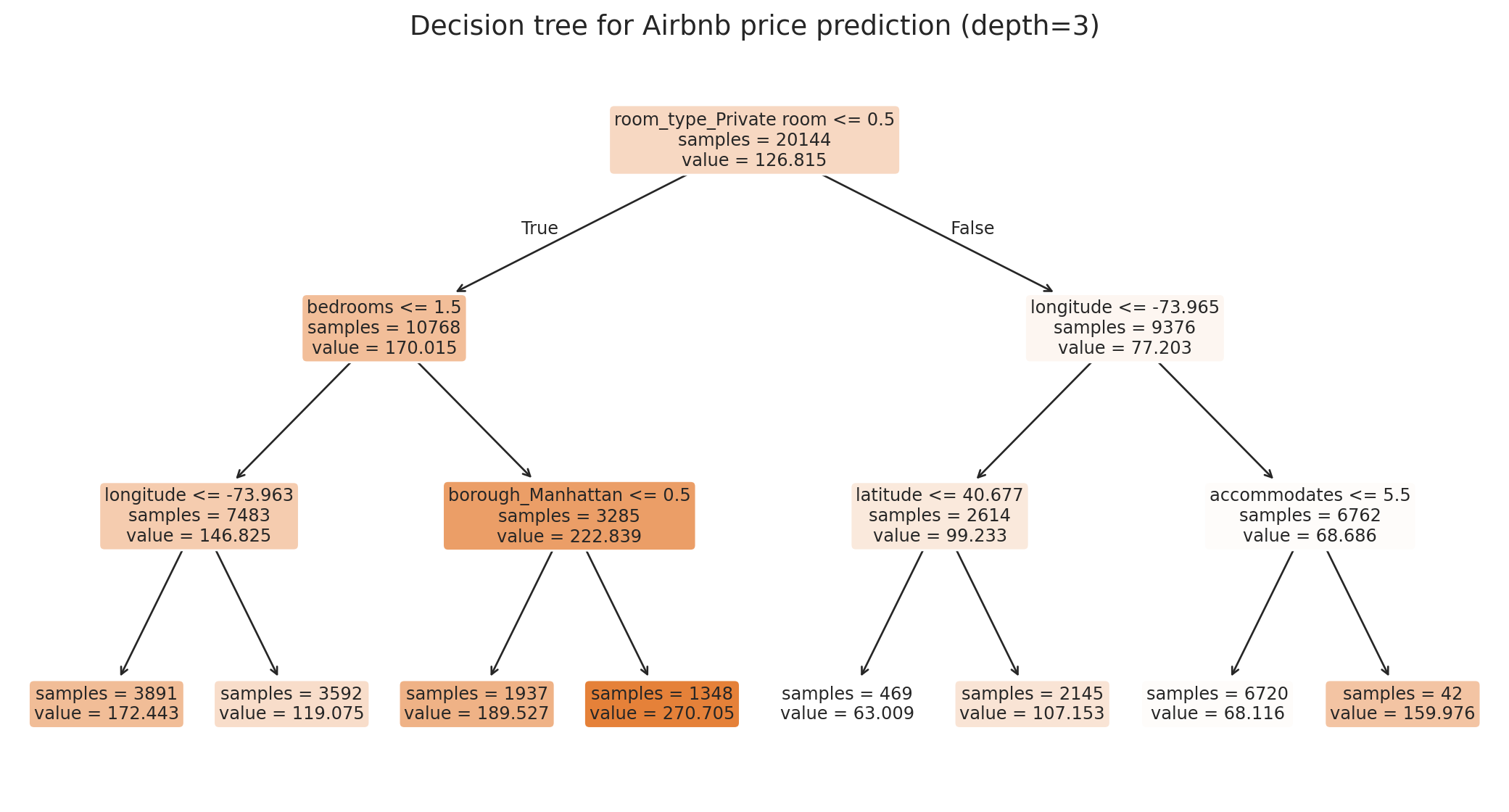
A decision tree splits the feature space into regions and predicts the mean price in each region. Each internal node asks an if/then question about one feature (“Is bedrooms > 2?”, “Is borough = Manhattan?”) and routes the observation left or right.

We hold out 30% of listings for honest evaluation (Chapter 6).

Code

X_train, X_test, y_train, y_test = train_test_split(
    X_base, prices, test_size=0.3, random_state=42
)

tree = DecisionTreeRegressor(max_depth=4, random_state=42)
tree.fit(X_train, y_train)

tree_train_r2 = tree.score(X_train, y_train)
tree_test_r2 = tree.score(X_test, y_test)

print(f"Decision Tree (depth=4):")
print(f"  Train R² = {tree_train_r2:.3f}  |  Test R² = {tree_test_r2:.3f}")

Decision Tree (depth=4):
  Train R² = 0.561  |  Test R² = 0.559

Think About It

Before running the next cell, predict: which feature lands at the root — bedrooms, room_type, or borough? Which appears second on the more expensive side?

Code

# Refit at depth=3 just for readability; depth-4 above is what we evaluate
tree_viz = DecisionTreeRegressor(max_depth=3, random_state=42)
tree_viz.fit(X_train, y_train)

fig, ax = plt.subplots(figsize=(11, 6))
plot_tree(tree_viz, feature_names=feature_names, filled=True, fontsize=9,
          rounded=True, ax=ax, impurity=False, proportion=False)
ax.set_title('Decision tree for Airbnb price prediction (depth=3)', fontsize=14)
plt.tight_layout()
plt.show()

Each leaf shows the predicted price and the sample count. The tree discovered on its own that room type and borough matter — no hand-crafted interactions, no specifying which neighborhoods to group.

Tree vocabulary

Reading the figure above:

Leaf — a node with no children. Each leaf stores one prediction: the mean training price of the observations that land there.
Internal node — any non-leaf node; asks a yes/no rule and sends each observation to one of two children.
Root — the single internal node at the top, where the first split happens.
Depth — the length of the longest root-to-leaf path; the max_depth argument caps it.

How a decision tree splits

A decision tree partitions the feature space using a greedy algorithm (greedy: chooses the locally best split at each step without planning ahead). At each node, it considers every feature and every possible threshold, choosing the split that produces the most homogeneous child nodes.

The criterion for “most homogeneous” is the sum of squared errors (SSE) in the two child regions:

\[\min_{j,\, s} \left[ \sum_{x_i \in R_1(j,s)} (y_i - \bar{y}_1)^2 + \sum_{x_i \in R_2(j,s)} (y_i - \bar{y}_2)^2 \right]\]

where each leaf predicts the mean $\bar{y}$ of its training observations. The same procedure runs recursively inside each child until a stopping criterion (max depth, minimum leaf size) kicks in.

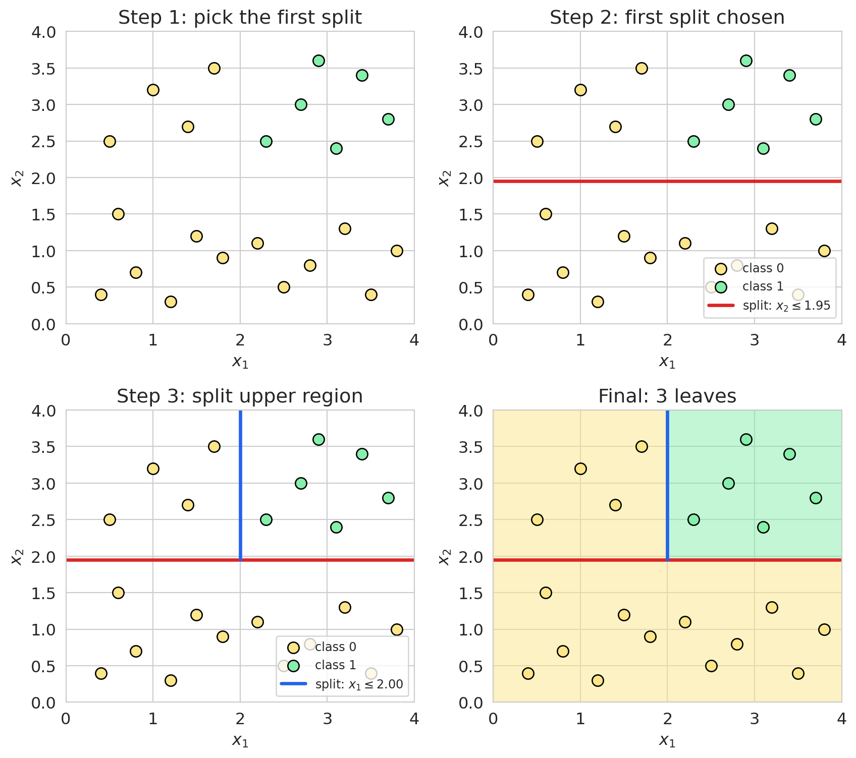
A worked example on a tiny dataset

Easier to see recursive partitioning than to read it. A 2D toy dataset with 22 points in two colors — yellow strip along the bottom, yellow cluster upper-left, green cluster upper-right. Fit a depth-2 tree and watch it split.

Code

toy_X = np.array([
    [0.4, 0.4], [0.8, 0.7], [1.2, 0.3], [1.5, 1.2], [1.8, 0.9],   # bottom strip
    [2.2, 1.1], [2.5, 0.5], [2.8, 0.8], [3.2, 1.3], [3.5, 0.4],
    [3.8, 1.0], [0.6, 1.5],
    [0.5, 2.5], [1.0, 3.2], [1.4, 2.7], [1.7, 3.5],               # upper-left
    [2.3, 2.5], [2.7, 3.0], [3.1, 2.4], [3.4, 3.4], [3.7, 2.8], [2.9, 3.6],  # upper-right
])
toy_y = np.array([0]*12 + [0]*4 + [1]*6)
toy_clf = DecisionTreeClassifier(max_depth=2, random_state=42).fit(toy_X, toy_y)

tt = toy_clf.tree_
root_feat, root_thr = tt.feature[0], tt.threshold[0]
right_node = tt.children_right[0]
right_feat, right_thr = tt.feature[right_node], tt.threshold[right_node]

fig, axes = plt.subplots(2, 2, figsize=(9, 8))
axes = axes.ravel()

def scatter_pts(ax):
    ax.scatter(toy_X[toy_y==0, 0], toy_X[toy_y==0, 1], s=70, c='#fde68a',
               edgecolors='black', linewidth=1, label='class 0')
    ax.scatter(toy_X[toy_y==1, 0], toy_X[toy_y==1, 1], s=70, c='#86efac',
               edgecolors='black', linewidth=1, label='class 1')
    ax.set_xlim(0, 4); ax.set_ylim(0, 4)
    ax.set_xlabel('$x_1$'); ax.set_ylabel('$x_2$')

scatter_pts(axes[0])
axes[0].set_title('Step 1: pick the first split')

scatter_pts(axes[1])
axes[1].axhline(root_thr, color='#dc2626', linewidth=2.5,
                label=f'split: $x_{root_feat+1} \\leq {root_thr:.2f}$')
axes[1].set_title('Step 2: first split chosen')
axes[1].legend(loc='lower right', fontsize=9)

scatter_pts(axes[2])
axes[2].axhline(root_thr, color='#dc2626', linewidth=2.5)
axes[2].plot([right_thr, right_thr], [root_thr, 4], color='#2563eb', linewidth=2.5,
             label=f'split: $x_{right_feat+1} \\leq {right_thr:.2f}$')
axes[2].set_title('Step 3: split upper region')
axes[2].legend(loc='lower right', fontsize=9)

axes[3].fill_between([0, 4], 0, root_thr, color='#fde68a', alpha=0.5)
axes[3].fill_between([0, right_thr], root_thr, 4, color='#fde68a', alpha=0.5)
axes[3].fill_between([right_thr, 4], root_thr, 4, color='#86efac', alpha=0.5)
scatter_pts(axes[3])
axes[3].axhline(root_thr, color='#dc2626', linewidth=2.5)
axes[3].plot([right_thr, right_thr], [root_thr, 4], color='#2563eb', linewidth=2.5)
axes[3].set_title('Final: 3 leaves')

plt.tight_layout()
plt.show()

The first split (x_2 ≤ 1.95) peels the bottom strip off — that child is all one color. The upper child still mixes colors, so it gets a second split (x_1 ≤ 2.00) separating the upper-left yellow cluster from the upper-right green cluster. Three pure leaves.

Two things to notice. The algorithm is greedy — at each node it commits to the best split right now and never reconsiders. Greedy splitting is fast and standard practice, but not guaranteed optimal (the optimization is NP-hard in general). The splits are axis-aligned — every cut is parallel to an axis, so a single tree approximates a diagonal boundary with a staircase. We come back to this in §Trees vs. logistic regression.

The same depth-3 tree as text:

Code

print(export_text(tree_viz, feature_names=feature_names, max_depth=3))

|--- room_type_Private room <= 0.50
|   |--- bedrooms <= 1.50
|   |   |--- longitude <= -73.96
|   |   |   |--- value: [172.44]
|   |   |--- longitude >  -73.96
|   |   |   |--- value: [119.08]
|   |--- bedrooms >  1.50
|   |   |--- borough_Manhattan <= 0.50
|   |   |   |--- value: [189.53]
|   |   |--- borough_Manhattan >  0.50
|   |   |   |--- value: [270.71]
|--- room_type_Private room >  0.50
|   |--- longitude <= -73.97
|   |   |--- latitude <= 40.68
|   |   |   |--- value: [63.01]
|   |   |--- latitude >  40.68
|   |   |   |--- value: [107.15]
|   |--- longitude >  -73.97
|   |   |--- accommodates <= 5.50
|   |   |   |--- value: [68.12]
|   |   |--- accommodates >  5.50
|   |   |   |--- value: [159.98]

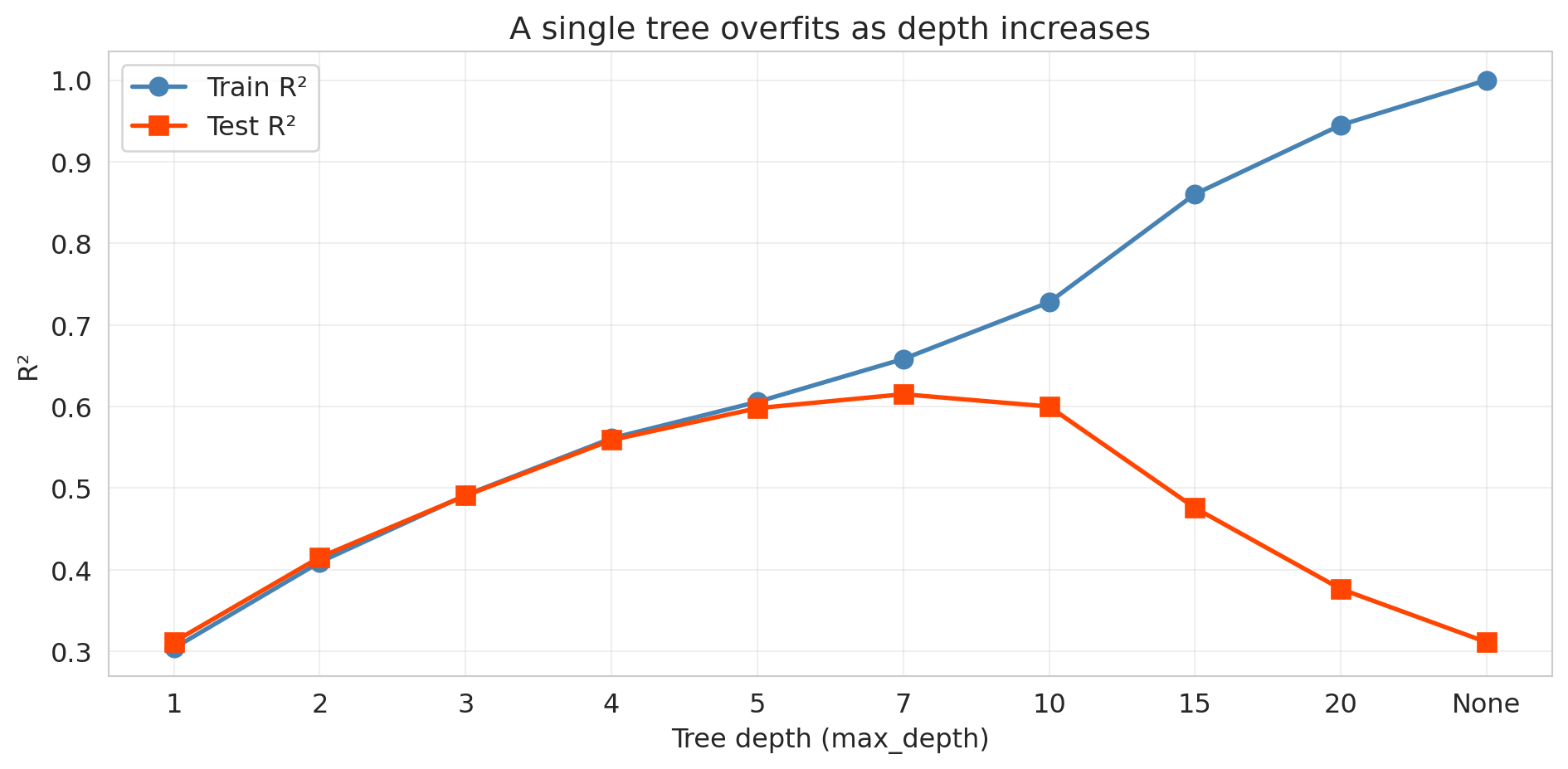
Overfitting a single tree

With no depth limit, a tree keeps splitting until every leaf holds a single observation. The next cell sweeps depth from 1 to None and tracks train vs. test R².

Predict before you verify

Sketch what you expect train R² to look like as depth grows, and what you expect test R² to look like. At what depth do you predict test R² peaks?

Code

depths = [1, 2, 3, 4, 5, 7, 10, 15, 20, None]
depth_labels = [str(d) if d else 'None' for d in depths]
train_r2s, test_r2s = [], []

for d in depths:
    t = DecisionTreeRegressor(max_depth=d, random_state=42).fit(X_train, y_train)
    train_r2s.append(t.score(X_train, y_train))
    test_r2s.append(t.score(X_test, y_test))
    print(f"depth={str(d):>4s}:  Train R² = {train_r2s[-1]:.3f}  |  Test R² = {test_r2s[-1]:.3f}")

fig, ax = plt.subplots(figsize=(10, 5))
x_pos = range(len(depths))
ax.plot(x_pos, train_r2s, 'o-', color='steelblue', linewidth=2, markersize=8, label='Train R²')
ax.plot(x_pos, test_r2s, 's-', color='orangered', linewidth=2, markersize=8, label='Test R²')
ax.set_xticks(x_pos); ax.set_xticklabels(depth_labels)
ax.set_xlabel('Tree depth (max_depth)'); ax.set_ylabel('R²')
ax.set_title('A single tree overfits as depth increases')
ax.legend(fontsize=12); ax.grid(True, alpha=0.3)
plt.tight_layout(); plt.show()

depth=   1:  Train R² = 0.304  |  Test R² = 0.312
depth=   2:  Train R² = 0.409  |  Test R² = 0.415
depth=   3:  Train R² = 0.491  |  Test R² = 0.491
depth=   4:  Train R² = 0.561  |  Test R² = 0.559
depth=   5:  Train R² = 0.606  |  Test R² = 0.598
depth=   7:  Train R² = 0.658  |  Test R² = 0.615
depth=  10:  Train R² = 0.728  |  Test R² = 0.600
depth=  15:  Train R² = 0.860  |  Test R² = 0.476
depth=  20:  Train R² = 0.945  |  Test R² = 0.376
depth=None:  Train R² = 1.000  |  Test R² = 0.311

Train R² climbs toward 1.0 while test R² peaks near depth 7 and collapses — the bias-variance tradeoff from Chapter 6. Shallow trees underfit (high bias, low variance); deep trees memorize noise (low bias, high variance). The “complexity knob” is now max_depth instead of polynomial degree.

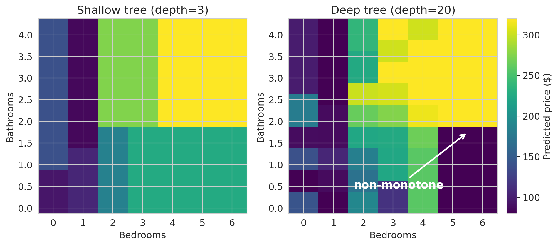
To see what shallow and deep trees actually predict, train each on just bedrooms and bathrooms and color a 2D grid by the predicted price.

Code

X_2d_train = X_train[['bedrooms', 'bathrooms']]

bed_grid  = np.arange(0, 7)
bath_grid = np.arange(0, 4.5, 0.25)
BB, AA = np.meshgrid(bed_grid, bath_grid)
X_grid_2d = pd.DataFrame({'bedrooms': BB.ravel(), 'bathrooms': AA.ravel()})

fig, axes = plt.subplots(1, 2, figsize=(11, 4.5))
vmin, vmax = 80, 320  # shared price scale so the panels are comparable

for ax, depth, title in zip(axes,
                            [3, 20],
                            ['Shallow tree (depth=3)', 'Deep tree (depth=20)']):
    t = DecisionTreeRegressor(max_depth=depth, random_state=42)
    t.fit(X_2d_train, y_train)
    preds = t.predict(X_grid_2d).reshape(BB.shape)
    im = ax.imshow(preds, origin='lower', aspect='auto', cmap='viridis',
                   vmin=vmin, vmax=vmax,
                   extent=[bed_grid.min() - 0.5, bed_grid.max() + 0.5,
                           bath_grid.min() - 0.125, bath_grid.max() + 0.125])
    ax.set_xlabel('Bedrooms'); ax.set_ylabel('Bathrooms'); ax.set_title(title)
    ax.set_xticks(bed_grid); ax.set_yticks(np.arange(0, 4.5, 0.5))

axes[1].annotate('non-monotone',
                 xy=(5.5, 1.75), xytext=(3.2, 0.45),
                 fontsize=14, color='white', fontweight='bold',
                 arrowprops=dict(arrowstyle='->', color='white', lw=2),
                 ha='center')

fig.colorbar(im, ax=axes.ravel().tolist(), label='Predicted price ($)',
             fraction=0.025, pad=0.02)
plt.show()

Both predictions are rectangular blocks of constant color — the tree’s signature. (A linear model would render the same plot as a smooth gradient.) The shallow tree carves a few orderly blocks: bigger listings cost more, every step of the way. The deep tree is a quilt of small rectangles where the gradient breaks — adjacent cells where adding a bedroom lowers the prediction (highlighted). The tree has memorized a few quirky training listings.

Think About It

A coworker proposes shipping a tree at max_depth=20 because “deeper is more flexible.” Using only the depth-vs-R² plot above, write a one-sentence rebuttal. Which depth would you ship instead, and what would you measure to defend the choice?

Choosing tree depth by cross-validation

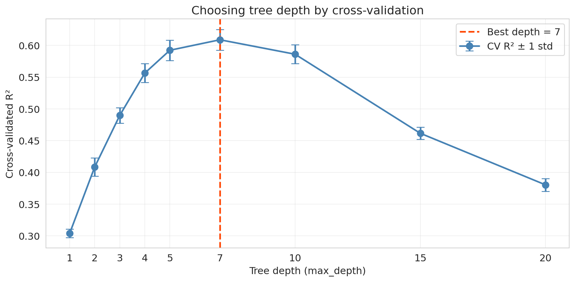
How do we pick the right depth? The same tool from Chapter 6: cross-validation. Sweep candidate depths, score each with 5-fold CV, take the best. Picking depth by peeking at the test set would burn the test set — CV does the tuning on training data, keeping the test set clean for a final honest report.

Code

depths_cv = [1, 2, 3, 4, 5, 7, 10, 15, 20]
cv_means, cv_stds = [], []

for d in depths_cv:
    scores = cross_val_score(DecisionTreeRegressor(max_depth=d, random_state=42),
                             X_train, y_train, cv=5, scoring='r2')
    cv_means.append(scores.mean()); cv_stds.append(scores.std())
    print(f"depth={d:>2d}: CV R² = {scores.mean():.4f} ± {scores.std():.4f}")

best_depth = depths_cv[np.argmax(cv_means)]
print(f"\nBest depth by CV: {best_depth}")

fig, ax = plt.subplots(figsize=(10, 5))
ax.errorbar(depths_cv, cv_means, yerr=cv_stds, fmt='o-', color='steelblue',
            linewidth=2, markersize=8, capsize=5, label='CV R² ± 1 std')
ax.axvline(best_depth, color='orangered', linestyle='--', linewidth=2,
           label=f'Best depth = {best_depth}')
ax.set_xlabel('Tree depth (max_depth)'); ax.set_ylabel('Cross-validated R²')
ax.set_title('Choosing tree depth by cross-validation')
ax.set_xticks(depths_cv)
ax.legend(fontsize=12); ax.grid(True, alpha=0.3)
plt.tight_layout(); plt.show()

depth= 1: CV R² = 0.3039 ± 0.0068
depth= 2: CV R² = 0.4084 ± 0.0143
depth= 3: CV R² = 0.4897 ± 0.0121
depth= 4: CV R² = 0.5563 ± 0.0149
depth= 5: CV R² = 0.5923 ± 0.0160
depth= 7: CV R² = 0.6088 ± 0.0164
depth=10: CV R² = 0.5861 ± 0.0149
depth=15: CV R² = 0.4615 ± 0.0094
depth=20: CV R² = 0.3803 ± 0.0101

Best depth by CV: 7

The U-shaped CV curve mirrors the polynomial experiment from Chapter 6. The same workflow picks any hyperparameter: lasso $\alpha$, polynomial degree, tree depth, number of neighbors — sweep, score by CV, take the best.

Think About It

The next section runs CV for classification instead of regression. Before reading on, predict the two substitutions you’d need to make in the loop above.

Code

best_tree = DecisionTreeRegressor(max_depth=best_depth, random_state=42)
best_tree.fit(X_train, y_train)
print(f"Tree at CV-best depth={best_depth}: Test R² = {best_tree.score(X_test, y_test):.3f}")

Tree at CV-best depth=7: Test R² = 0.615

Classification trees

Trees handle classification just as naturally. Swap squared error for Gini impurity; everything else — greedy recursive partitioning, depth control, cross-validation — is identical. Evaluation metrics (confusion matrix, precision, recall, ROC, AUC) are the same ones you used for logistic regression in Chapter 7.

Going deeper: Gini impurity

For a node with $K$ classes and class proportions $\hat p_1, \dots, \hat p_K$, the Gini index is

\[\text{Gini} = 1 - \sum_{k=1}^{K} \hat p_k^2,\]

which simplifies to $2\hat p(1-\hat p)$ in the binary case. A pure node has Gini = 0; a 50/50 binary node has Gini = 0.5. The tree picks splits that maximize the impurity drop $\text{Gini}_{\text{parent}} - p_L\, \text{Gini}_L - p_R\, \text{Gini}_R$ — the categorical analogue of “drop SSE the most.”

Create a binary target: is a listing “expensive” (price above $200)?

Code

y_train_exp = (y_train > 200).astype(int)
y_test_exp = (y_test > 200).astype(int)

print(f"Expensive listings: {y_train_exp.mean():.1%} of training set, "
      f"{y_test_exp.mean():.1%} of test set")

Expensive listings: 13.3% of training set, 13.3% of test set

Pick depth by cross-validation, same recipe as regression.

Code

depths_clf = [1, 2, 3, 4, 5, 7, 10, 15, 20]
cv_means_clf = []
for d in depths_clf:
    scores = cross_val_score(DecisionTreeClassifier(max_depth=d, random_state=42),
                             X_train, y_train_exp, cv=5, scoring='accuracy')
    cv_means_clf.append(scores.mean())
    print(f"depth={d:>2d}: CV accuracy = {scores.mean():.4f} ± {scores.std():.4f}")

best_depth_clf = depths_clf[np.argmax(cv_means_clf)]
print(f"\nBest depth by CV: {best_depth_clf}")

depth= 1: CV accuracy = 0.8665 ± 0.0001
depth= 2: CV accuracy = 0.8812 ± 0.0027
depth= 3: CV accuracy = 0.8925 ± 0.0033
depth= 4: CV accuracy = 0.8941 ± 0.0037
depth= 5: CV accuracy = 0.8986 ± 0.0035
depth= 7: CV accuracy = 0.9001 ± 0.0037
depth=10: CV accuracy = 0.8943 ± 0.0021
depth=15: CV accuracy = 0.8809 ± 0.0042
depth=20: CV accuracy = 0.8718 ± 0.0022

Best depth by CV: 7

Code

clf_tree = DecisionTreeClassifier(max_depth=best_depth_clf, random_state=42).fit(X_train, y_train_exp)
y_pred_tree = clf_tree.predict(X_test)
y_prob_tree = clf_tree.predict_proba(X_test)[:, 1]

print(f"Classification tree (depth={best_depth_clf}):")
print(f"  Accuracy  = {clf_tree.score(X_test, y_test_exp):.3f}")
print(f"  Precision = {precision_score(y_test_exp, y_pred_tree):.3f}")
print(f"  Recall    = {recall_score(y_test_exp, y_pred_tree):.3f}")
print(f"  F1        = {f1_score(y_test_exp, y_pred_tree):.3f}")
print(f"  AUC       = {roc_auc_score(y_test_exp, y_prob_tree):.3f}")

Classification tree (depth=7):
  Accuracy  = 0.896
  Precision = 0.668
  Recall    = 0.437
  F1        = 0.528
  AUC       = 0.908

Code

fpr_tree, tpr_tree, _ = roc_curve(y_test_exp, y_prob_tree)
auc_tree = roc_auc_score(y_test_exp, y_prob_tree)

fig, axes = plt.subplots(1, 2, figsize=(11, 4.5))
cm = confusion_matrix(y_test_exp, y_pred_tree)
ConfusionMatrixDisplay(cm, display_labels=['< $200', '≥ $200']).plot(
    ax=axes[0], cmap='Blues', values_format='d')
axes[0].set_title(f'Classification tree (depth={best_depth_clf})')

axes[1].plot(fpr_tree, tpr_tree, color='steelblue', linewidth=2.5,
             label=f'Classification tree (AUC = {auc_tree:.3f})')
axes[1].plot([0, 1], [0, 1], 'k--', linewidth=1, label='Random guess')
axes[1].set_xlabel('False positive rate'); axes[1].set_ylabel('True positive rate (recall)')
axes[1].set_title('ROC curve — classification tree')
axes[1].legend(fontsize=11); axes[1].grid(True, alpha=0.3)
plt.tight_layout(); plt.show()

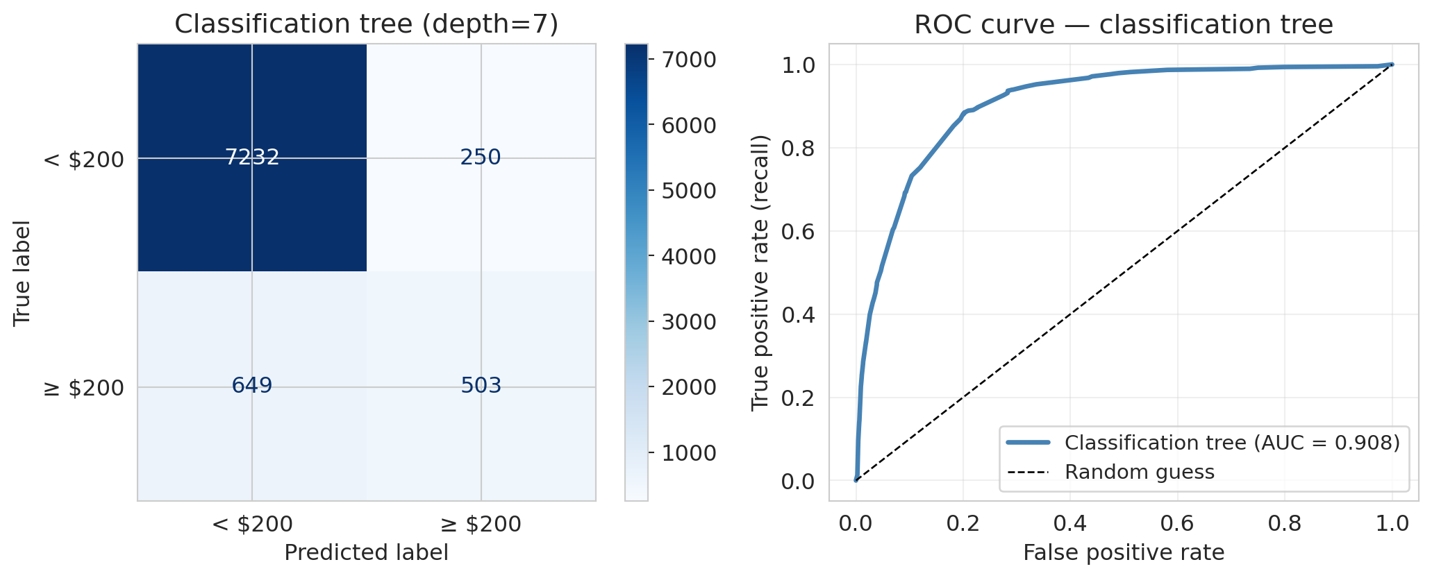
If you understand regression trees, you understand classification trees — same splits (room type, borough, bedrooms), now routing to “expensive” or “not expensive” leaves.

Random forests

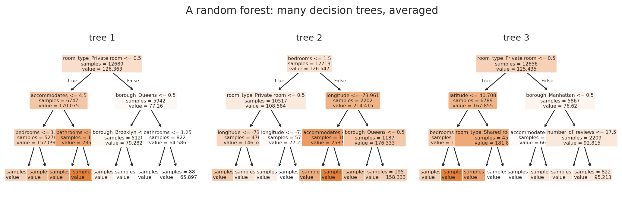
A random forest fits hundreds of decision trees, each on a random subset of the data and features, and averages their predictions. Each tree captures the same underlying signal but memorizes different noise, so averaging preserves the signal and shrinks the variance.

Code

forest_demo = RandomForestRegressor(n_estimators=3, max_depth=3, min_samples_leaf=50,
                                    max_features=0.3,
                                    random_state=11, n_jobs=-1).fit(X_train, y_train)

fig, axes = plt.subplots(1, 3, figsize=(11, 3.5))
for i, ax in enumerate(axes):
    plot_tree(forest_demo.estimators_[i], feature_names=feature_names, filled=True,
              fontsize=6, rounded=True, ax=ax, impurity=False, proportion=False)
    ax.set_title(f'tree {i+1}', fontsize=11)
fig.suptitle('A random forest: many decision trees, averaged', fontsize=13)
plt.tight_layout()
plt.show()

Three trees from a tiny random forest. Each tree sees a different bootstrap sample of rows and considers different features at each split, so they split differently. The forest’s prediction is the average of all the trees.

Code

rf = RandomForestRegressor(n_estimators=100, min_samples_leaf=5,
                           random_state=42, n_jobs=-1).fit(X_train, y_train)
rf_test_r2 = rf.score(X_test, y_test)

print("Model comparison (test R²):")
print(f"  Decision Tree (depth=4):     {tree_test_r2:.3f}")
print(f"  Random Forest (100 trees):   {rf_test_r2:.3f}")

Model comparison (test R²):
  Decision Tree (depth=4):     0.559
  Random Forest (100 trees):   0.657

The forest beats the single tree. n_estimators=100 is the number of trees; min_samples_leaf=5 requires each leaf to hold at least 5 training rows, so trees can capture structure but no single leaf depends on two or three quirky bootstrap rows.

How random forests work: bagging + feature subsampling

A random forest combines two ideas:

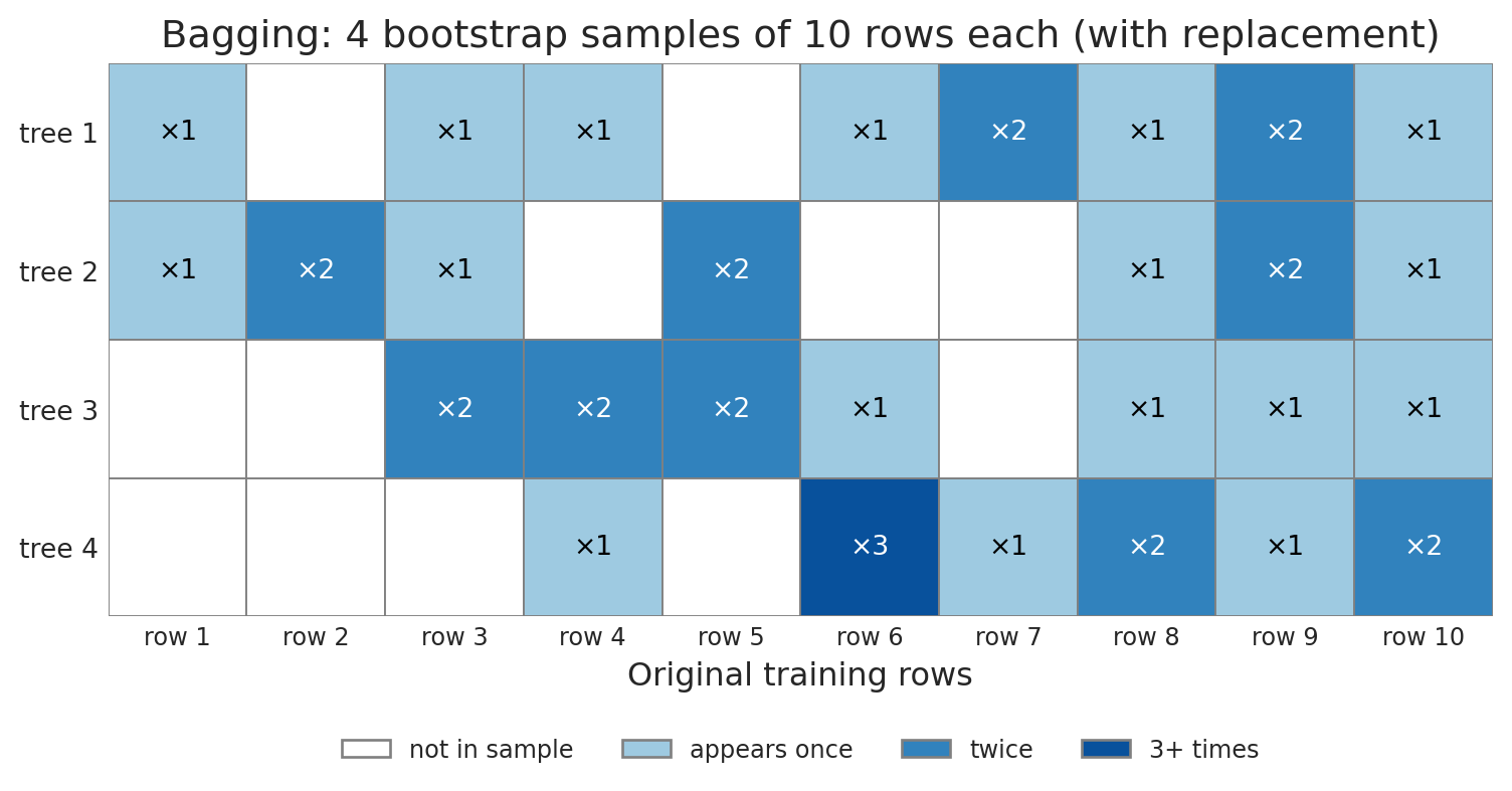
Bagging (bootstrap aggregating): each tree trains on a bootstrap sample — same size as the original dataset, drawn with replacement. So a 3-row dataset $(A, B, C)$ might yield $(A, B, B)$ or $(C, C, A)$.
Feature subsampling: at each split, the tree considers only a random subset of features (default $\sqrt{p}$ for classification, a larger fraction for regression).¹ Limiting each split forces trees to find different splits, decorrelating them.

The ensemble prediction averages tree predictions (regression) or takes majority vote (classification). Each tree memorizes different noise from its own bootstrap sample, so averaging shrinks the variance.

Going deeper: out-of-bag samples

A bootstrap sample of size $n$ from $n$ rows includes ~63% of distinct rows; the other 37% are out-of-bag (OOB). Each tree’s error on its OOB rows averages to a near-unbiased estimate of generalization error — cross-validation for free. Set oob_score=True in RandomForestRegressor.

Ensembles, more generally

A random forest is one instance of an ensemble: a model built by aggregating many weaker learners into a stronger predictor. Two strategies dominate, distinguished by how the learners are produced:

Bagging (parallel) — train learners independently on bootstrap samples; average. Mechanism: variance reduction.
Boosting (sequential) — train learners one at a time, each focused on previous mistakes; combine as a weighted sum. Mechanism: bias reduction. Gradient boosting — fits each new learner to the residuals — is treated in Chapter 17.

Ensembling turns a moderately good model into a much better one without hand-engineering features. It is the reason “use a random forest” is the strong tabular-data default.

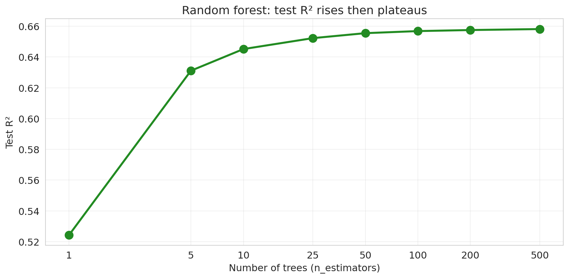
More trees rarely hurt

Train random forests with increasing numbers of trees and track test performance.

Code

n_trees_list = [1, 5, 10, 25, 50, 100, 200, 500]
rf_test_scores = []

for n_trees in n_trees_list:
    rf_temp = RandomForestRegressor(n_estimators=n_trees, min_samples_leaf=5,
                                    random_state=42, n_jobs=-1).fit(X_train, y_train)
    rf_test_scores.append(rf_temp.score(X_test, y_test))
    print(f"n_estimators = {n_trees:>3d}: Test R² = {rf_test_scores[-1]:.4f}")

fig, ax = plt.subplots(figsize=(10, 5))
ax.plot(n_trees_list, rf_test_scores, 'o-', color='forestgreen', linewidth=2.5, markersize=10)
ax.set_xlabel('Number of trees (n_estimators)'); ax.set_ylabel('Test R²')
ax.set_title('Random forest: test R² rises then plateaus')
ax.set_xscale('log'); ax.set_xticks(n_trees_list); ax.set_xticklabels(n_trees_list)
ax.grid(True, alpha=0.3); plt.tight_layout(); plt.show()

n_estimators =   1: Test R² = 0.5243
n_estimators =   5: Test R² = 0.6311
n_estimators =  10: Test R² = 0.6452
n_estimators =  25: Test R² = 0.6523
n_estimators =  50: Test R² = 0.6555
n_estimators = 100: Test R² = 0.6569
n_estimators = 200: Test R² = 0.6575
n_estimators = 500: Test R² = 0.6582

No U-shape — test R² rises and plateaus. In expectation, adding more trees improves or matches performance; you may see tiny dips in any one run from finite-sample noise. (Caveat: this is specific to bagging. For gradient boosting (Chapter 17), too many trees can overfit.)

Escaping the classical U-curve

This is the “one known escape” promised by Chapter 6‘s Beyond the classical tradeoff callout. The classical U-shape assumes you are fitting a single model. A forest is an average over hundreds: as long as individual trees’ errors are sufficiently uncorrelated, adding more trees drives variance down without pushing bias up. The U-curve in max_depth is replaced by a one-sided staircase in n_estimators.

Individual trees are overfit; their average has lower variance

In 1906, Francis Galton watched 787 villagers guess the weight of an ox at a country fair. Their median guess was 1207 pounds; the actual weight was 1198 — within 1%, even though individual guesses varied wildly.² Bagging plays the same trick on overfit trees: each tree memorizes different noise from its own bootstrap sample, and averaging shrinks the spread toward the truth.

Code

n_rows, n_samples = 10, 4
rng = np.random.default_rng(7)
bag_idx = rng.integers(0, n_rows, size=(n_samples, n_rows))

fig, ax = plt.subplots(figsize=(8, 4))
colors = {0: 'white', 1: '#9ecae1', 2: '#3182bd', 3: '#08519c'}
for s in range(n_samples):
    counts = np.bincount(bag_idx[s], minlength=n_rows)
    for r, c in enumerate(counts):
        c_clip = min(int(c), 3)
        ax.add_patch(plt.Rectangle((r, n_samples - 1 - s), 1, 1,
                                   facecolor=colors[c_clip], edgecolor='gray', linewidth=0.7))
        if c >= 1:
            ax.text(r + 0.5, n_samples - 1 - s + 0.5, f'×{c}',
                    ha='center', va='center', fontsize=10,
                    color='white' if c >= 2 else 'black')

ax.set_xlim(0, n_rows); ax.set_ylim(0, n_samples)
ax.set_xticks(np.arange(n_rows) + 0.5)
ax.set_xticklabels([f'row {i+1}' for i in range(n_rows)], fontsize=9)
ax.set_yticks(np.arange(n_samples) + 0.5)
ax.set_yticklabels([f'tree {n_samples - i}' for i in range(n_samples)], fontsize=10)
ax.set_xlabel('Original training rows')
ax.set_title('Bagging: 4 bootstrap samples of 10 rows each (with replacement)')
ax.set_aspect('equal')
for spine in ax.spines.values(): spine.set_visible(False)
ax.tick_params(axis='both', length=0)

from matplotlib.patches import Patch
legend_elems = [Patch(facecolor='white', edgecolor='gray', label='not in sample'),
                Patch(facecolor='#9ecae1', edgecolor='gray', label='appears once'),
                Patch(facecolor='#3182bd', edgecolor='gray', label='twice'),
                Patch(facecolor='#08519c', edgecolor='gray', label='3+ times')]
ax.legend(handles=legend_elems, loc='upper center',
          bbox_to_anchor=(0.5, -0.18), ncol=4, fontsize=9, frameon=False)
plt.tight_layout()
plt.show()

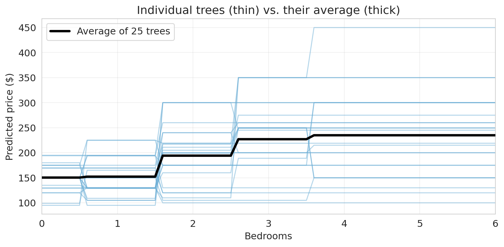
Each tree sees a different bootstrap sample of the rows; some rows appear multiple times, some not at all.

To see this on actual trees, train 25 deep trees on bootstrap samples and plot their predictions along a 1D slice (price vs. bedrooms, other features at median).

Code

median_features = X_train.median()
bedroom_range = np.arange(0, 7, 0.1)
X_slice = pd.DataFrame(
    np.tile(median_features.values, (len(bedroom_range), 1)),
    columns=X_train.columns
)
X_slice['bedrooms'] = bedroom_range

rng = np.random.default_rng(42)
pool_size, n_show = 200, 25
pool_preds = np.empty((pool_size, len(bedroom_range)))
for i in range(pool_size):
    boot_idx = rng.integers(0, len(X_train), size=len(X_train))
    tree_i = DecisionTreeRegressor(max_depth=None, random_state=i)
    tree_i.fit(X_train.iloc[boot_idx], y_train.iloc[boot_idx])
    pool_preds[i] = tree_i.predict(X_slice)

fig, ax = plt.subplots(figsize=(9, 4.5))
for i in range(n_show):
    ax.plot(bedroom_range, pool_preds[i], alpha=0.5, linewidth=1.2, color='#6baed6')
ax.plot(bedroom_range, pool_preds[:n_show].mean(axis=0), color='black', linewidth=3,
        label=f'Average of {n_show} trees', zorder=5)
ax.set_xlabel('Bedrooms'); ax.set_ylabel('Predicted price ($)')
ax.set_title('Individual trees (thin) vs. their average (thick)')
ax.legend(loc='upper left'); ax.set_xlim(0, 6); ax.grid(True, alpha=0.3)
plt.tight_layout(); plt.show()

Individual trees wiggle as the bedroom count changes — each one memorizes different noise from its own bootstrap sample. The thick black line, their average, is much steadier: where the individual trees disagree, the disagreements partly cancel.

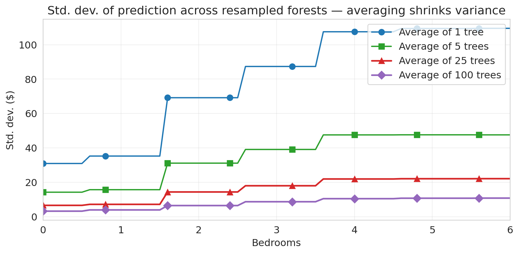
To make “steadier” precise, repeat the experiment for forests of different sizes. For each $B \in \{1, 5, 25, 100\}$, sample $B$ trees with replacement, average their predictions, and record the standard deviation across many such samples.

Code

# For each B, compute std across the means of B trees sampled with replacement.
def stability(B, preds, n_groups=200, seed=0):
    rng_ = np.random.default_rng(seed)
    group_means = np.stack([
        preds[rng_.choice(preds.shape[0], size=B, replace=True)].mean(axis=0)
        for _ in range(n_groups)
    ])
    return group_means.std(axis=0)

fig, ax = plt.subplots(figsize=(9, 4.5))
B_styles = [(1, '#1f77b4', 'o', 1.6), (5, '#2ca02c', 's', 1.6),
            (25, '#d62728', '^', 2.0), (100, '#9467bd', 'D', 2.0)]
for B, color, marker, lw in B_styles:
    ax.plot(bedroom_range, stability(B, pool_preds),
            color=color, linewidth=lw, marker=marker, markevery=8, markersize=7,
            label=f'Average of {B} tree' + ('s' if B > 1 else ''))
ax.set_xlabel('Bedrooms')
ax.set_ylabel('Std. dev. ($)')
ax.set_title('Std. dev. of prediction across resampled forests — averaging shrinks variance')
ax.legend(loc='upper right'); ax.set_xlim(0, 6); ax.grid(True, alpha=0.3)
plt.tight_layout(); plt.show()

A single tree swings by tens of dollars across bootstrap samples; each $4\times$ more trees roughly halves the spread, and the curves bend toward a floor as the trees become correlated.

The floor is the punchline: averaging only helps when trees make independent mistakes. Feature subsampling forces trees to find different splits, decorrelating them and lowering the floor.

Going deeper: the variance-of-an-average formula

The variance of an average of $B$ trees, where $\sigma^2$ is one tree’s prediction variance and $\rho$ is the average pairwise correlation, is

\[\text{Var}(\bar f_B) = \rho \sigma^2 + \frac{1-\rho}{B}\sigma^2.\]

The $1-\rho$ term shrinks like $1/B$ (so the standard deviation shrinks like $1/\sqrt{B}$ — what the bottom panel plots). The $\rho \sigma^2$ floor does not depend on $B$; feature subsampling beats it down by lowering $\rho$. Returns in Chapter 17.

Averaging shrinks the spread of the prediction without shifting its center. A random forest keeps each tree deep (low bias) and reduces variance by averaging, replacing the U-curve in max_depth with a one-sided staircase in n_estimators.

Random forest as benchmark

Compare the random forest’s test R² to the hand-engineered linear model from Chapter 5. To make the comparison interesting, hand the linear model the bedrooms × borough interactions from Chapter 5; the forest gets only the raw feature matrix.

Code

# Linear model with interactions (same as Chapter 5)
borough_dummies = pd.get_dummies(df['borough'], drop_first=True)
interactions = borough_dummies.multiply(df['bedrooms'], axis=0)
interactions.columns = [f'bedrooms_x_{col}' for col in interactions.columns]
X_interact = pd.concat([X_base, interactions], axis=1)

lm_simple = LinearRegression().fit(X_train, y_train)
lm_simple_test_r2 = r2_score(y_test, lm_simple.predict(X_test))

lm_interact = LinearRegression().fit(
    X_interact.loc[X_train.index], y_train
)
lm_interact_test_r2 = r2_score(y_test, lm_interact.predict(X_interact.loc[X_test.index]))

print("Test R² comparison:")
print(f"  Linear model (bedrooms + bath + room + borough):  {lm_simple_test_r2:.3f}")
print(f"  Linear model + interactions:                      {lm_interact_test_r2:.3f}")
print(f"  Decision tree (depth=4):                          {tree_test_r2:.3f}")
print(f"  Random forest (100 trees):                        {rf_test_r2:.3f}")

Test R² comparison:
  Linear model (bedrooms + bath + room + borough):  0.571
  Linear model + interactions:                      0.576
  Decision tree (depth=4):                          0.559
  Random forest (100 trees):                        0.657

Surprise

The random forest wins with no manual feature engineering — no hand-crafted polynomial terms, no interactions the analyst had to pick. (Trees do build interactions internally: each split refines the partition produced by the splits above it. The point is that the forest discovers which features and combinations to use without analyst guidance.) For tabular prediction, a forest is a strong default benchmark: if your hand-crafted model can’t beat it, the engineering effort may not be worthwhile.

Think About It

The forest beats the linear model with interactions. Does that mean linear models are useless? What advantages might a linear model still have?

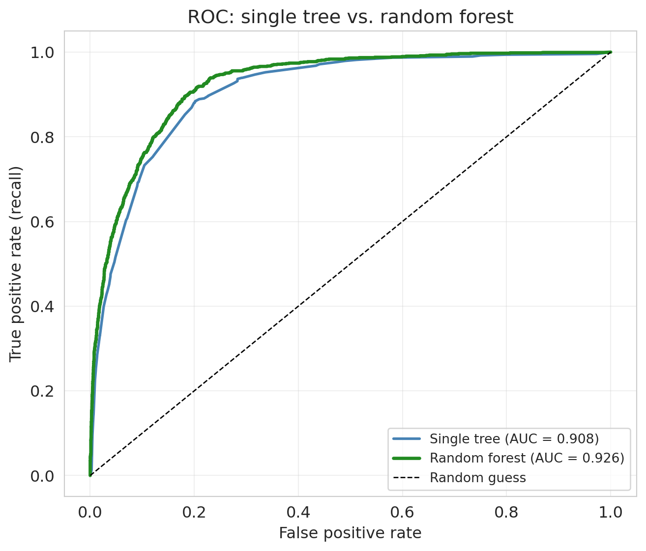
Random forest classifier

Same recipe for classification: bag deep trees, average their probability estimates. Use the classifier-flavored loss (log-loss instead of squared error) and evaluate with AUC.

Code

rf_clf = RandomForestClassifier(n_estimators=100, min_samples_leaf=5,
                                random_state=42, n_jobs=-1).fit(X_train, y_train_exp)
y_pred_rf = rf_clf.predict(X_test)
y_prob_rf = rf_clf.predict_proba(X_test)[:, 1]
fpr_rf, tpr_rf, _ = roc_curve(y_test_exp, y_prob_rf)
auc_rf = roc_auc_score(y_test_exp, y_prob_rf)

fig, ax = plt.subplots(figsize=(7, 6))
ax.plot(fpr_tree, tpr_tree, color='steelblue', linewidth=2,
        label=f'Single tree (AUC = {auc_tree:.3f})')
ax.plot(fpr_rf, tpr_rf, color='forestgreen', linewidth=2.5,
        label=f'Random forest (AUC = {auc_rf:.3f})')
ax.plot([0, 1], [0, 1], 'k--', linewidth=1, label='Random guess')
ax.set_xlabel('False positive rate'); ax.set_ylabel('True positive rate (recall)')
ax.set_title('ROC: single tree vs. random forest')
ax.legend(fontsize=10); ax.grid(True, alpha=0.3)
plt.tight_layout(); plt.show()

AUC rises from 0.908 (single tree) to 0.926 (forest) — the forest’s ROC sits above the single tree’s at nearly every threshold.

Trees vs. logistic regression

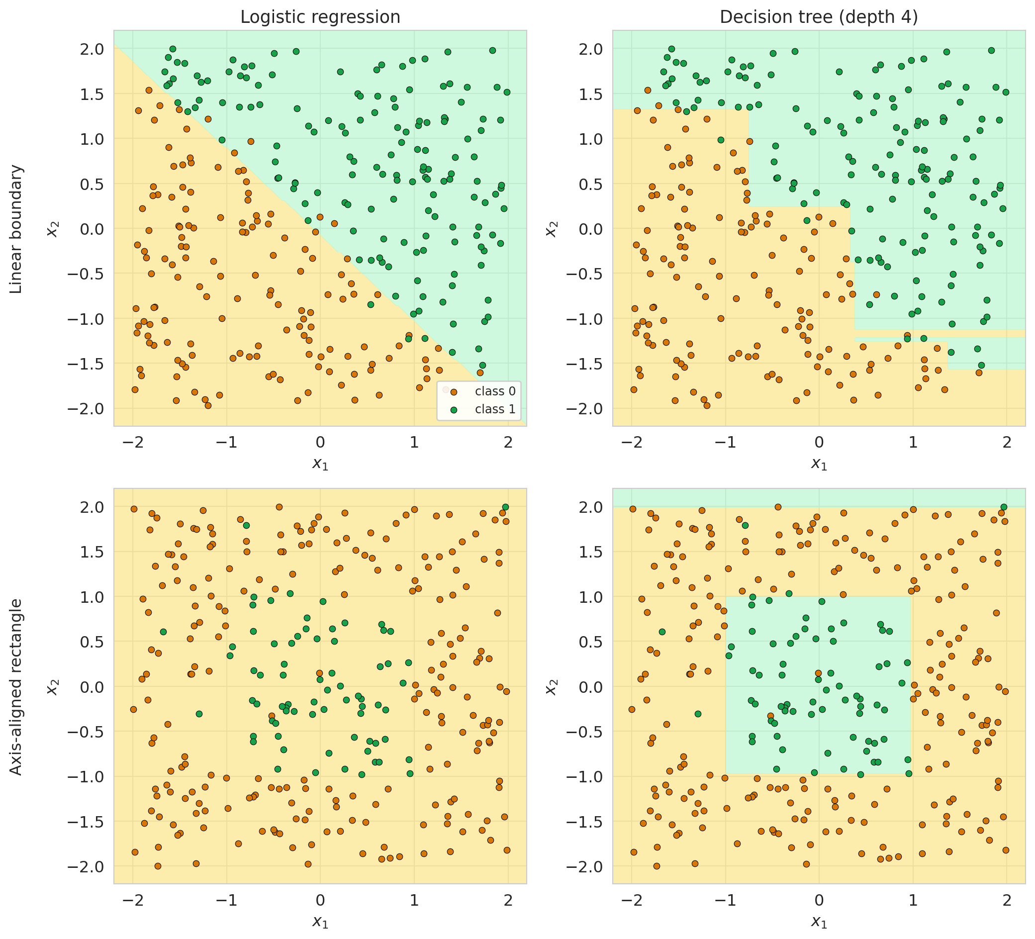
We now have two classification approaches: trees and logistic regression from Chapter 7. The right model is a property of the data, not the model family. Below: two synthetic problems — a linear boundary (top) and an axis-aligned rectangle (bottom) — fit with logistic regression and a depth-4 tree.

Code

rng = np.random.default_rng(42)

# Linear: y=1 above x1+x2=0, with a small noise band.
X_lin = rng.uniform(-2, 2, size=(300, 2))
y_lin = ((X_lin[:, 0] + X_lin[:, 1] + 0.3 * rng.standard_normal(300)) > 0).astype(int)

# Box: y=1 inside the unit square, with 5% label flips.
X_box = rng.uniform(-2, 2, size=(300, 2))
y_box = ((X_box[:, 0] > -1) & (X_box[:, 0] < 1) &
        (X_box[:, 1] > -1) & (X_box[:, 1] < 1)).astype(int)
y_box = np.where(rng.random(300) < 0.05, 1 - y_box, y_box)

xx, yy = np.meshgrid(np.linspace(-2.2, 2.2, 200), np.linspace(-2.2, 2.2, 200))
grid = np.c_[xx.ravel(), yy.ravel()]

fig, axes = plt.subplots(2, 2, figsize=(11, 10))
rows = [(X_lin, y_lin, 'Linear boundary'),
        (X_box, y_box, 'Axis-aligned rectangle')]
cols = [('Logistic regression', LogisticRegression(max_iter=1000)),
        ('Decision tree (depth 4)', DecisionTreeClassifier(max_depth=4, random_state=42))]

for i, (X_dat, y_dat, dname) in enumerate(rows):
    for j, (mname, mdl) in enumerate(cols):
        ax = axes[i, j]
        m = mdl.__class__(**mdl.get_params()).fit(X_dat, y_dat)
        Z = m.predict(grid).reshape(xx.shape)
        ax.contourf(xx, yy, Z, levels=[-0.5, 0.5, 1.5],
                    colors=['#fde68a', '#bbf7d0'], alpha=0.7)
        ax.scatter(X_dat[y_dat == 0, 0], X_dat[y_dat == 0, 1],
                   s=22, c='#d97706', edgecolors='black', linewidth=0.4,
                   label='class 0' if (i == 0 and j == 0) else None)
        ax.scatter(X_dat[y_dat == 1, 0], X_dat[y_dat == 1, 1],
                   s=22, c='#16a34a', edgecolors='black', linewidth=0.4,
                   label='class 1' if (i == 0 and j == 0) else None)
        if i == 0: ax.set_title(mname, fontsize=13)
        ax.set_ylabel(f'{dname}\n\n$x_2$' if j == 0 else '$x_2$', fontsize=12 if j == 0 else None)
        ax.set_xlabel('$x_1$')

axes[0, 0].legend(loc='lower right', fontsize=9, framealpha=0.9)
plt.tight_layout()
plt.show()

Linear loses on the rectangle; tree loses on the diagonal. Linear models are good at smooth, monotone effects, bad at corners and interactions. Trees are good at corners, thresholds, and interactions, bad at smooth diagonals (a single slope becomes a staircase). On real data you don’t know which geometry the truth has — fit both and compare held-out performance.

Now the same comparison on Airbnb.

Code

from sklearn.preprocessing import StandardScaler
from sklearn.pipeline import Pipeline

# Logistic regression with L2 needs scaled inputs (our features mix scales).
lr = Pipeline([
    ('scale', StandardScaler()),
    ('logreg', LogisticRegression(max_iter=1000, random_state=42)),
]).fit(X_train, y_train_exp)

y_pred_lr = lr.predict(X_test)
y_prob_lr = lr.predict_proba(X_test)[:, 1]
fpr_lr, tpr_lr, _ = roc_curve(y_test_exp, y_prob_lr)
auc_lr = roc_auc_score(y_test_exp, y_prob_lr)

Code

print(f"{'Metric':<12} {'Logistic Reg':>14} {'Tree (d={})'.format(best_depth_clf):>14} {'RF (100)':>14}")
print("-" * 58)
for name, fn in [('Precision', precision_score), ('Recall', recall_score), ('F1', f1_score)]:
    print(f"{name:<12} {fn(y_test_exp, y_pred_lr):>14.3f} "
          f"{fn(y_test_exp, y_pred_tree):>14.3f} "
          f"{fn(y_test_exp, y_pred_rf):>14.3f}")
print(f"{'AUC':<12} {auc_lr:>14.3f} {auc_tree:>14.3f} {auc_rf:>14.3f}")

Metric         Logistic Reg     Tree (d=7)       RF (100)
----------------------------------------------------------
Precision             0.720          0.668          0.737
Recall                0.415          0.437          0.453
F1                    0.526          0.528          0.561
AUC                   0.912          0.908          0.926

Code

fig, ax = plt.subplots(figsize=(8, 6))
ax.plot(fpr_lr, tpr_lr, color='darkorange', linewidth=2.5,
        label=f'Logistic regression (AUC = {auc_lr:.3f})')
ax.plot(fpr_tree, tpr_tree, color='steelblue', linewidth=2,
        label=f'Classification tree (AUC = {auc_tree:.3f})')
ax.plot(fpr_rf, tpr_rf, color='forestgreen', linewidth=2.5,
        label=f'Random forest (AUC = {auc_rf:.3f})')
ax.plot([0, 1], [0, 1], 'k--', linewidth=1, label='Random guess')
ax.set_xlabel('False positive rate')
ax.set_ylabel('True positive rate (recall)')
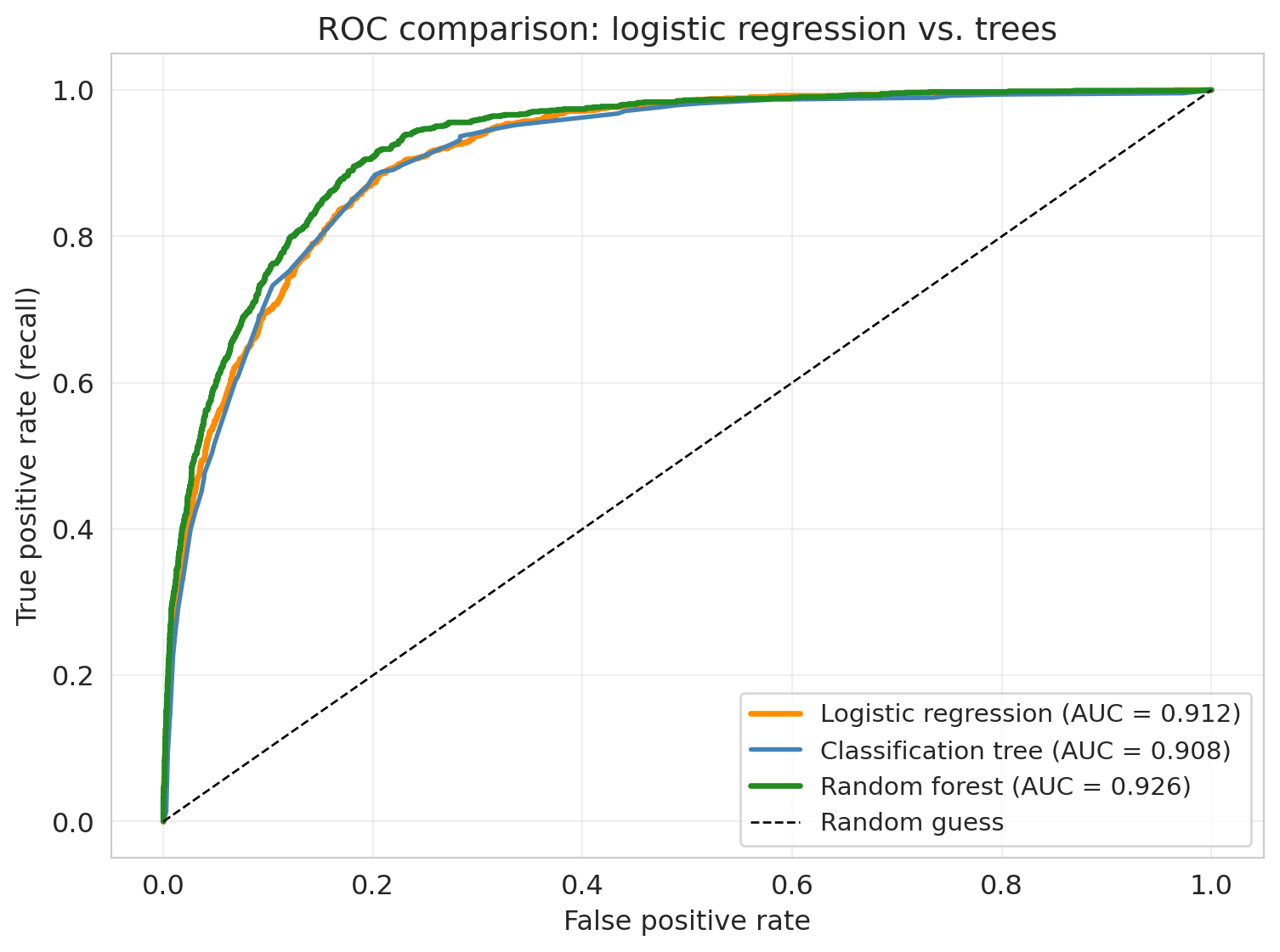
ax.set_title('ROC comparison: logistic regression vs. trees')
ax.legend(fontsize=11)
ax.grid(True, alpha=0.3)
plt.tight_layout()
plt.show()

Each approach has distinct strengths:

Logistic regression — interpretable coefficients (log-odds per feature: each bedroom multiplies the odds of expensive by $e^{\beta}$). Fast, stable, works when the true boundary is roughly linear.
Decision trees — capture nonlinearities and interactions without feature engineering. A tree can learn “Manhattan + 2+ bedrooms = expensive” on its own. Easy to visualize.
Random forests — nonlinear power plus variance reduction. Harder to interpret, but consistently strong on tabular data with minimal tuning.

Prefer logistic regression for interpretability or small datasets; prefer trees/forests for many features with potential interactions when per-feature coefficients aren’t needed.

Think About It

You’ve now seen all four cells of the linear-vs-trees × regression-vs-classification grid. Pick one of these scenarios and decide which model family you’d reach for first, and why:

A health-insurance underwriter wants to price policies and produce, for each applicant, a one-line explanation of which factors moved their premium up or down.
A music app suspects that users who listened to 5+ artists in a particular genre AND created 2+ playlists are upgrade-prone — but only on certain device types. The team wants a model that can discover this kind of behavioral threshold-and-interaction rule from hundreds of usage signals without specifying the cuts in advance.
A small clinic wants to flag charts likely to contain a coding error before billing, working from 40 fields where most patients are missing 5–10 of them.

Feature importance

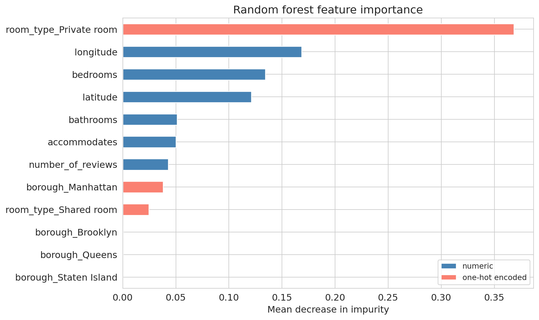
A random forest is harder to interpret than linear regression — no single coefficient says “each bedroom adds $X.” But it does report which features it relies on most.

Feature importance measures how much each feature contributes to reducing prediction error across all trees. Sklearn’s feature_importances_ reports mean decrease in impurity (MDI): for each split, the impurity drop is weighted by the share of samples flowing through that node, summed within each tree, averaged, and normalized to sum to 1.

Code

importances = pd.Series(rf.feature_importances_, index=feature_names)
importances_sorted = importances.sort_values()

# Color by feature type to preview the MDI-bias warning below.
numeric_features = {'latitude', 'longitude', 'accommodates', 'bedrooms',
                    'bathrooms', 'number_of_reviews'}
bar_colors = ['steelblue' if f in numeric_features else 'salmon'
              for f in importances_sorted.index]

fig, ax = plt.subplots(figsize=(10, 6))
importances_sorted.plot(kind='barh', ax=ax, color=bar_colors, edgecolor='white')
ax.set_xlabel('Mean decrease in impurity')
ax.set_title('Random forest feature importance')

from matplotlib.patches import Patch
ax.legend(handles=[Patch(facecolor='steelblue', label='numeric'),
                   Patch(facecolor='salmon', label='one-hot encoded')],
          loc='lower right', fontsize=10)
plt.tight_layout()
plt.show()

Linear regression’s bedrooms coefficient tells you the marginal effect of one extra bedroom — a causal-flavored interpretation (under strong assumptions). Feature importance tells you something different: how much the forest uses a feature for splitting, reflecting direct effects and interactions. A feature can be important without a simple linear relationship.

Going deeper: permutation importance

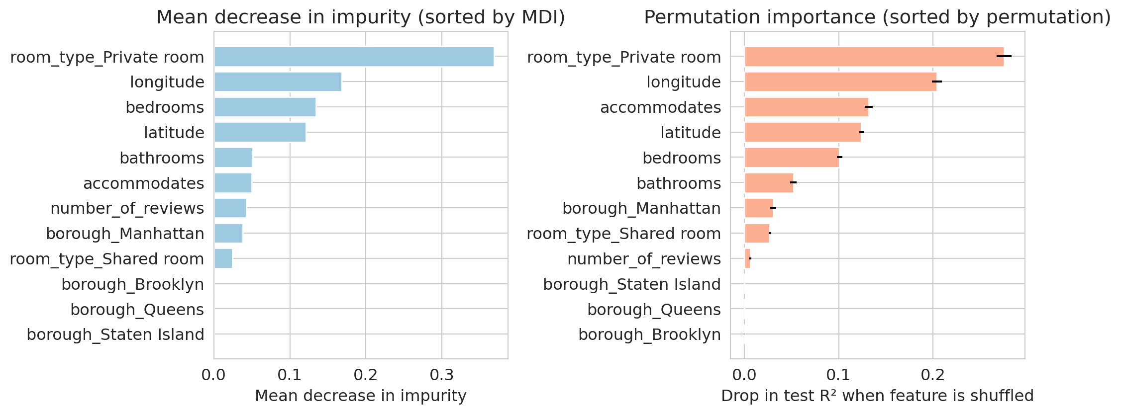
MDI has a known bias: it favors high-cardinality features (a continuous column has hundreds of split-point chances; a binary one has one). Two features with equal predictive signal can rank very differently on MDI just because of cardinality.

Permutation importance is model-agnostic: if I randomly shuffle column $j$, how much worse does the model do on held-out data? Shuffling a useful column hurts; shuffling a useless one doesn’t.

Code

from sklearn.inspection import permutation_importance

# Use held-out test set so the score reflects generalization.
perm = permutation_importance(rf, X_test, y_test, n_repeats=10,
                              random_state=42, n_jobs=-1, scoring='r2')

imp_df = pd.DataFrame({'feature': feature_names,
                       'mdi': rf.feature_importances_,
                       'perm_mean': perm.importances_mean,
                       'perm_std': perm.importances_std})

# Each panel sorted by its own metric so rank-disagreement is visible.
mdi_sorted = imp_df.sort_values('mdi')
perm_sorted = imp_df.sort_values('perm_mean')

fig, axes = plt.subplots(1, 2, figsize=(11, 4.5))
axes[0].barh(mdi_sorted['feature'], mdi_sorted['mdi'],
             color='#9ecae1', edgecolor='white')
axes[0].set_xlabel('Mean decrease in impurity')
axes[0].set_title('Mean decrease in impurity (sorted by MDI)')

axes[1].barh(perm_sorted['feature'], perm_sorted['perm_mean'],
             xerr=perm_sorted['perm_std'],
             color='#fcae91', edgecolor='white')
axes[1].set_xlabel('Drop in test R² when feature is shuffled')
axes[1].set_title('Permutation importance (sorted by permutation)')

plt.tight_layout()
plt.show()

Compare the two panels: features re-rank. accommodates rises under permutation, bedrooms slips. MDI credits every split equally; permutation only credits features that actually drive generalization. Two practical rules: compute permutation importance on held-out data, and watch correlated features — if two columns share signal, shuffling either alone can look unimportant since the model leans on the other. Drop correlated groups in or out together.

How trees handle missing data

Unlike linear regression — which needs complete data for every row — trees handle missing values directly. A tree’s yes/no questions just need a rule for which branch missing values follow; linear models break entirely without a numeric value to multiply.

Modern tree implementations — including the popular gradient-boosting libraries XGBoost and LightGBM, and (since scikit-learn 1.3) sklearn’s own DecisionTreeRegressor/Classifier — learn at each split which child missing-valued rows go to, picking whichever direction reduces the loss more. No imputation needed.

Going deeper: XGBoost vs. LightGBM

Both XGBoost and LightGBM fit gradient-boosted trees (rather than the bagged trees that make up a random forest — see Chapter 17). Both handle missing values natively. Both win Kaggle leaderboards. They differ in how they grow each tree.

XGBoost grows trees level by level (balanced trees, predictable training time, forgiving defaults). The conservative default — start here.
LightGBM grows trees leaf by leaf (asymmetric, deeper trees, more aggressive fitting) and bins continuous features into histograms — dramatically faster on large datasets.

Rule of thumb: reach for XGBoost first; switch to LightGBM when training time hurts (millions of rows or hundreds of features → often 5–10× faster). Either beats RandomForestRegressor on most tabular benchmarks because boosting reduces bias (Chapter 17). Sklearn’s HistGradientBoostingRegressor/Classifier is a fine third option — one fewer install.

Think About It

If 30% of bedrooms is missing and you impute with the median before fitting a tree, what information have you destroyed? Would the tree have been better off seeing the missingness?

In practice, tree-based models (especially gradient-boosted) are the standard choice for tabular data with missing values — they don’t force the analyst into imputation decisions that could bias the answer.

When to doubt the forest

A strong test score on tabular data does not address three limitations.

Distribution shift. Each prediction is the mean training $y$ inside one leaf, so a forest cannot output a value outside the range of the training $y$ values. For inputs unlike anything seen at training — a new neighborhood, a post-pandemic price regime — the leaf they route into may have no relationship to the new input. Chapter 6’s distribution-shift caveats apply.
Feature importance is descriptive, not causal. A high MDI on accommodates means the forest used that variable for many splits — not that increasing capacity would raise price. Permutation importance has the same limitation.
Correlated features share importance. If bedrooms and accommodates carry overlapping signal, the forest can lean on either, so each one’s importance is split between them. Interpret correlated features as a group.

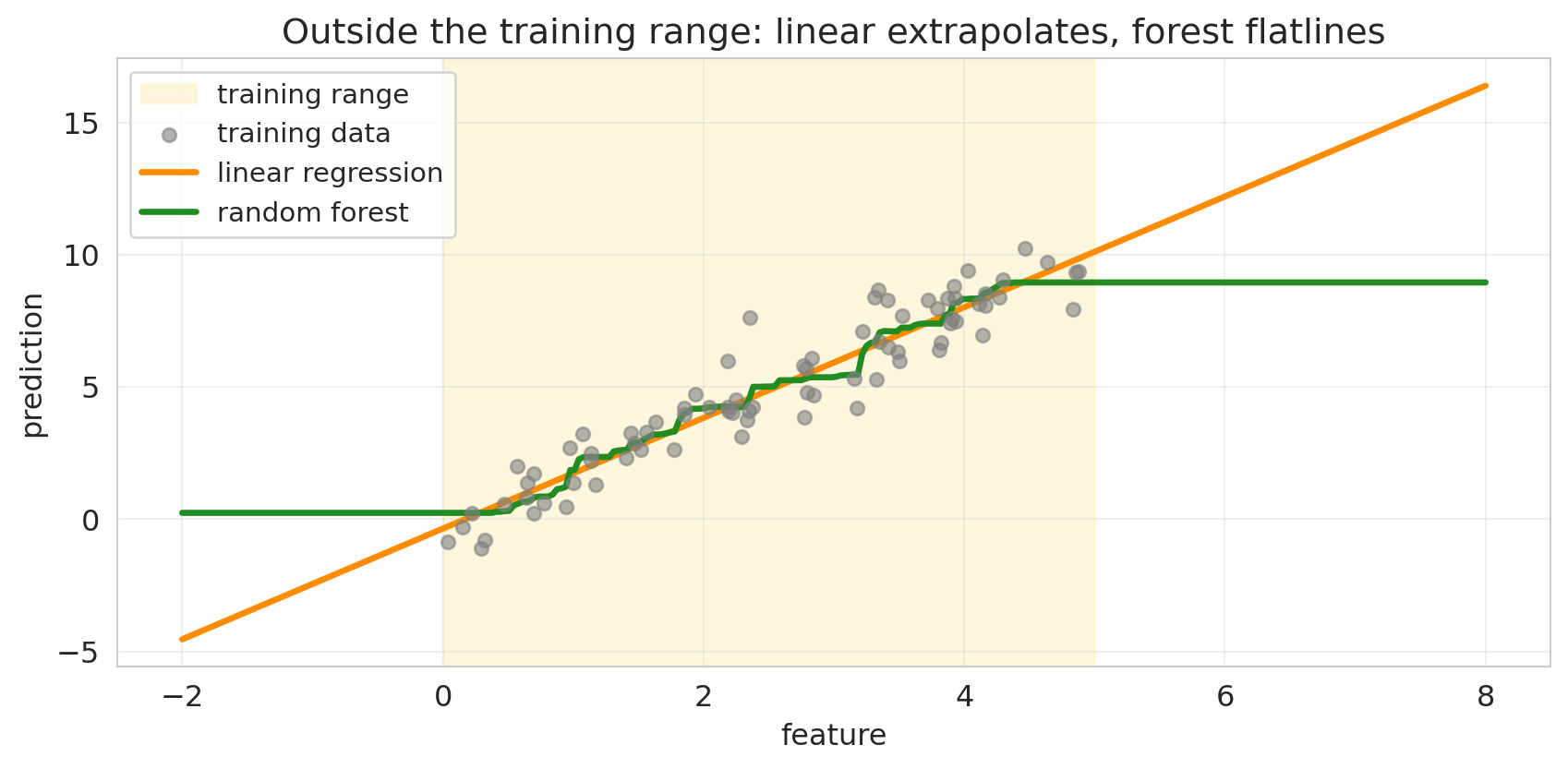
Distribution shift: linear extrapolates, forest flatlines

To see how a forest behaves outside its training range, fit both a linear regression and a random forest on the same 1D training data, then ask each to predict on a wider range.

Code

rng_ext = np.random.default_rng(42)
n = 80
x_demo = rng_ext.uniform(0, 5, size=n).reshape(-1, 1)
y_demo = 2 * x_demo.ravel() + rng_ext.normal(0, 1, n)

lr_demo = LinearRegression().fit(x_demo, y_demo)
rf_demo = RandomForestRegressor(n_estimators=200, min_samples_leaf=5,
                                random_state=42, n_jobs=-1).fit(x_demo, y_demo)

x_wide = np.linspace(-2, 8, 300).reshape(-1, 1)
fig, ax = plt.subplots(figsize=(9, 4.5))
ax.axvspan(0, 5, color='#fef3c7', alpha=0.6, label='training range', zorder=0)
ax.scatter(x_demo, y_demo, s=30, color='gray', alpha=0.6,
           label='training data', zorder=3)
ax.plot(x_wide, lr_demo.predict(x_wide), color='darkorange', linewidth=2.5,
        label='linear regression')
ax.plot(x_wide, rf_demo.predict(x_wide), color='forestgreen', linewidth=2.5,
        label='random forest')
ax.set_xlabel('feature'); ax.set_ylabel('prediction')
ax.set_title('Outside the training range: linear extrapolates, forest flatlines')
ax.legend(loc='upper left', fontsize=11)
ax.grid(True, alpha=0.3)
plt.tight_layout(); plt.show()

The linear model extends its fitted slope past the training range. The forest predicts a constant — the mean training $y$ of whichever leaf the input routes into. Whether the linear extrapolation is right depends on whether the underlying relationship really is linear outside the training range; the forest’s flatline is never right outside, by construction.

Correlated features in numbers

bedrooms and accommodates are strongly correlated on Airbnb — most multi-bedroom listings also accommodate more guests. Permutation importance shuffles one feature and measures the drop in test $R^2$. Shuffling one of a correlated pair barely hurts, because the forest leans on the other.

Code

def shuffle_drop(cols, X, y, model, n_repeats=10, base_seed=0):
    drops = []
    for r in range(n_repeats):
        rng_ = np.random.default_rng(base_seed + r)
        X_shuf = X.copy()
        for c in cols:
            X_shuf[c] = rng_.permutation(X_shuf[c].values)
        drops.append(model.score(X, y) - model.score(X_shuf, y))
    return float(np.mean(drops))

corr_bed_acc = X_train['bedrooms'].corr(X_train['accommodates'])
drop_bed = shuffle_drop(['bedrooms'], X_test, y_test, rf)
drop_acc = shuffle_drop(['accommodates'], X_test, y_test, rf)
drop_both = shuffle_drop(['bedrooms', 'accommodates'], X_test, y_test, rf)

print(f"Correlation(bedrooms, accommodates) = {corr_bed_acc:.2f}\n")
print(f"Drop in test R² when we shuffle:")
print(f"  bedrooms only:                       {drop_bed:.3f}")
print(f"  accommodates only:                   {drop_acc:.3f}")
print(f"  bedrooms AND accommodates together:  {drop_both:.3f}")
print(f"\nSum of individual drops:           {drop_bed + drop_acc:.3f}")
print(f"Group drop / sum of individual:    {drop_both / (drop_bed + drop_acc):.1f}×")

Correlation(bedrooms, accommodates) = 0.64

Drop in test R² when we shuffle:
  bedrooms only:                       0.102
  accommodates only:                   0.132
  bedrooms AND accommodates together:  0.285

Sum of individual drops:           0.234
Group drop / sum of individual:    1.2×

Shuffling either feature alone costs the forest some R², because each carries unique signal beyond the other. But shuffling both together costs more than the sum: the shared signal hides when measured one-at-a-time, since the forest can lean on whichever feature isn’t shuffled. With more strongly correlated features (near-duplicates), the effect gets dramatic — each one looks nearly useless alone, while the group is essential. The fix is to read importance for correlated groups, not single columns.

Trust the predictions only on inputs that resemble the training data, and read the importance chart as a description of model usage, not a causal claim.

Back to the host

Friday’s prototype: ship the forest. It beats your hand-engineered linear model with no manual feature crosses, and it handles missing rooms, boroughs, and review counts without imputation choices that bias the answer. Set up drift monitoring on the inputs — a forest cannot extrapolate to new neighborhoods or new price regimes. And don’t present the importance chart as causal: it tells the host what the model used, not what raises a price.

Key takeaways

Decision trees find splits automatically — no manual feature engineering. The model examines every feature and every threshold, choosing greedy axis-aligned splits that minimize prediction error. The same algorithm — swap squared error for Gini impurity — handles classification.
A single deep tree overfits. With no depth limit, a tree memorizes the training data: training R² climbs toward 1.0 while test R² collapses.
Cross-validation picks the depth. The same 5-fold CV recipe used for polynomial degree and lasso $\alpha$ — sweep candidate values, score each, take the best — selects tree depth too.
Random forests average overfit trees, and the average is stable. Bagging plus feature subsampling decorrelates the trees, so averaging them reduces variance without raising bias. Adding more trees rarely hurts — no U-curve in n_estimators.
Trees vs. linear models is a geometry choice. Linear models excel on smooth, monotone effects; trees excel on corners, thresholds, and interactions. Forests beat hand-crafted linear models on prediction, but pay for it in interpretability — and the feature importance chart is descriptive, not causal.

Study guide

Key ideas

Decision tree — recursively partitions feature space by greedy if/then splits; predicts mean outcome (regression) or majority class (classification) per leaf.
Gini impurity — classification splitting criterion $1 - \sum_k \hat p_k^2$ (binary: $2\hat p(1-\hat p)$); replaces squared error when the target is categorical.
Bagging — train many models on bootstrap samples, average. Reduces variance without raising bias.
Feature subsampling — restrict each split to a random subset of features. Decorrelates trees so averaging works harder.
Random forest — bagged trees with feature subsampling. In expectation, more trees improves or matches performance — no U-curve in n_estimators.
Ensembles — bagging (parallel, variance reduction) vs. boosting (sequential, bias reduction; Chapter 17).
Feature importance (MDI) — mean decrease in impurity per feature, averaged across trees. Biased toward high-cardinality features; permutation importance is more robust.
Missing data in trees — handled natively via learned routing (XGBoost, LightGBM, recent sklearn) or surrogate splits (CART).
Trees vs. logistic regression — logistic gives interpretable coefficients; trees capture nonlinearities and interactions without feature engineering. Forests trade interpretability for strong default performance.

Computational tools

DecisionTreeRegressor(max_depth=4).fit(X, y) / DecisionTreeClassifier(max_depth=5).fit(X, y) — fits a tree with controlled depth.
RandomForestRegressor(n_estimators=100).fit(X, y) / RandomForestClassifier(...) — fits a forest.
plot_tree(tree, feature_names=..., filled=True) / export_text(tree, ...) — visualize/print tree rules.
rf.feature_importances_ — MDI scores.
confusion_matrix, roc_curve, roc_auc_score — classifier evaluation (Chapter 7).
train_test_split(X, y, test_size=0.3) and cross_val_score(model, X, y, cv=5) — for honest evaluation and depth selection.

For the quiz

You are responsible for: how a decision tree splits, why deep trees overfit, how bagging and feature subsampling combine to form a random forest, why more trees rarely hurts, feature importance interpretation, how trees handle missing data, cross-validation for tree depth, Gini impurity, and the tradeoffs between trees and logistic regression.

How was this chapter? Help us improve these notes. Share feedback

Leo Breiman introduced random forests in 2001 (“Random Forests”, Machine Learning 45:5–32) and coined “bagging” in 1996.↩︎
Galton, “Vox Populi”, Nature 75, 450–451 (1907).↩︎