---
title: "Permutation Tests"
execute:
enabled: true
jupyter: python3
---
```{python}
import numpy as np
import pandas as pd
import matplotlib.pyplot as plt
import seaborn as sns
from scipy import stats
import warnings
warnings.filterwarnings('ignore')
sns.set_style('whitegrid')
plt.rcParams['figure.figsize'] = (8, 5)
plt.rcParams['font.size'] = 12

DATA_DIR = 'data'
np.random.seed(42)
```
In [Chapter 8](lec08-sampling.qmd) we built a 95% bootstrap confidence interval for the ACTG treatment effect: $[39.6, 61.3]$, excluding zero. That interval already answers the usual question. "Does the drug have *any* effect?" becomes "is zero inside the interval?" If it isn't, the data rule out zero at the 5% level — and we can stop.
So why an entire chapter on **hypothesis testing**? Two reasons.
- **History:** Fisher's p-value (1925) predates Neyman's confidence interval (1937) by more than a decade.
- **Generality:** the permutation test extends to questions where no CI is natural — categorical outcomes, orderings, comparisons of whole distributions.
Both the bootstrap and the permutation test are examples of **simulation-based inference**: we build the reference distribution by resampling, not by deriving it from a closed-form formula.
:::{.callout-note}
## The Lady Tasting Tea
At Rothamsted Experimental Station in the 1920s, the algae researcher Muriel Bristol claimed she could taste whether milk had been added to a teacup before or after the tea. R.A. Fisher, a prolific contributor to the modern field of statistics — also at Rothamsted — took her seriously and designed a test: eight cups, four of each kind, presented in random order, with Bristol asked to pick out the four milk-first cups.
Fisher's insight was to ask what *pure guessing* would look like. There are $\binom{8}{4} = 70$ ways to pick four cups out of eight, and only one pick is the correct labeling — so a guesser hits the right answer about 1 time in 70, roughly a 1.4% chance. Bristol's actual result forces a choice between two stories: a middling result — a couple cups mixed up — looks like what we'd expect from guessing, and we'd keep the "she can't really tell" story; a spot-on result leaves us choosing between "she genuinely can taste the difference" and "we just watched a 1-in-70 coincidence." (Bristol got all eight cups right. See Fisher 1935 for the original design, or Salsburg 2001 for the historical account.)
:::
## Setup: the treatment effect
Let's move to a more modern example reload the ACTG 175 clinical trial data. In [Chapter 8](lec08-sampling.qmd), we estimated the difference of population means between the two groups — about 50 CD4 cells. In a clinical trial, this difference is called the **treatment effect**. (In ACTG 175, the "control" arm was AZT monotherapy and the "treatment" arm pools three more aggressive regimens — so the question the permutation test answers is *does the combination beat AZT alone?*, not *does the drug beat a placebo?* In 1991, giving a placebo to HIV+ patients with declining CD4 counts would have been ethically unacceptable.)
```{python}
df = pd.read_csv(f'{DATA_DIR}/clinical-trial/ACTG175.csv')
df['cd4_change'] = df['cd420'] - df['cd40']

control = df[df['treat'] == 0]['cd4_change']
treatment = df[df['treat'] == 1]['cd4_change']
n_T, n_C = len(treatment), len(control)

observed_effect = treatment.mean() - control.mean()
print(f"Control mean    (n_C = {n_C}): {control.mean():.1f} CD4 cells")
print(f"Treatment mean  (n_T = {n_T}): {treatment.mean():.1f} CD4 cells")
print(f"Observed effect:               {observed_effect:.1f} CD4 cells")
```
The bootstrap CI from [Chapter 8](lec08-sampling.qmd) was entirely above zero — suggestive that the drug works. Can we quantify exactly how surprising the data would be if the drug did nothing?
## The permutation test idea
**If the drug has no effect, group assignment is irrelevant.** The treatment label carries no information — every patient's outcome would be the same regardless of which group they were assigned to. This claim is the **null hypothesis**: the default assumption a test tries to disprove. The number we compute from the data to measure the effect (here, the difference of group means) is the **test statistic**.
So what happens if we **shuffle the labels**? If the null is true, reassigning patients at random should produce test statistics that look just like the observed one. If the observed statistic is much larger than what shuffling produces, that is evidence against the null.
:::{.callout-important}
## Definition: Permutation test
A hypothesis test that builds the **null distribution** by shuffling group labels and recomputing the test statistic. The null distribution shows what the test statistic would look like if the null hypothesis were true.
:::
Two terms, similar names, different jobs: the **null hypothesis** is a claim about the world ("the drug has no effect"); the **null distribution** is the distribution of the test statistic *if* that claim were true. The permutation test builds the second from the first by shuffling.
Why does shuffling simulate the null distribution? ACTG 175 randomized patients to treatment by coin flip. *Under the null of no effect*, a patient's CD4 change is determined by the patient alone, not by which arm they happened to get — so any relabeling is just as plausible as the original. The labels are **exchangeable**, and each shuffle is a draw from the same data-generating story as the real trial. (If the drug *does* work, shuffling mixes responders and non-responders, and the shuffled datasets look very different from the original — that difference is what the test detects.)
Random assignment guarantees exchangeability under the null. Exchangeability is the logical foundation of the permutation test.
:::{.callout-note collapse="true"}
## Going deeper: what exchangeability and "no effect" really mean
Two formalities hide behind the casual phrasings in this section.
**Exchangeability** is a property of the random variables, not of the labels. A sequence $(X_1, \ldots, X_n)$ is **exchangeable** when permuting the indices leaves the joint distribution unchanged: for any permutation $\pi$, $(X_{\pi(1)}, \ldots, X_{\pi(n)})$ has the same distribution as the original. Under the null of no effect, the data viewed through relabelings are exchangeable — which is what lets us read off the null distribution by shuffling.
**Sharp null vs equal-means null.** "No effect" is ambiguous. Fisher's **sharp null** says every patient's CD4 change is *exactly* what it would have been under either label — a strong per-patient claim. Neyman's weaker **equal-means null** says only that the two arms have the same expected CD4 change. The permutation test's validity requires the *sharp* null: a drug that left means unchanged but doubled the variance would satisfy equal-means but break exchangeability, and the test would reject spuriously. In most practical settings the distinction is invisible, but careful inference sits on the sharp null.
:::
### Step by step
1. Combine all CD4 changes into one pool (ignoring labels)
2. Randomly assign $n_C$ patients to "control" and the rest to "treatment"
3. Compute the test statistic (difference in means) on the fake groups
4. Repeat many times
```{python}
# Combine all CD4 changes into one pool
all_cd4 = np.concatenate([treatment.values, control.values])
print(f"Total patients: {len(all_cd4)}   (n_T = {n_T}, n_C = {n_C})")
```
Now we write a function that performs one permutation: it shuffles the combined data using `np.random.permutation()`, splits into two fake groups, and returns the difference of group means.
```{python}
def permutation_diff_of_means(values, n_first):
    """One shuffle: the first `n_first` entries become group A, the rest group B.
    Returns mean(A) − mean(B)."""
    shuffled = np.random.permutation(values)
    return shuffled[:n_first].mean() - shuffled[n_first:].mean()

print("Five random permutations (treatment − control):")
for i in range(5):
    fake = permutation_diff_of_means(all_cd4, n_T)
    print(f"  Permutation {i+1}: fake effect = {fake:+.1f} CD4 cells")

print(f"\nObserved effect:                          {observed_effect:+.1f} CD4 cells")
```
The fake effects bounce around zero — small positive, small negative. Our observed effect of ~50 looks very different.
:::{.callout-tip}
## Think about it
You're on the FDA advisory panel. The observed treatment effect is ~50 CD4 cells; the fake effects we just saw ranged roughly from −7 to +7. Before seeing the full null distribution, what fraction of fake effects *greater than or equal to 50* would you need to see to vote against the drug? 1 in 100? 1 in 1,000? 1 in a million? There is no right answer here — the exercise is to commit to a standard *before* the data comes in. Sanity check your answer by asking: would you be comfortable defending your threshold to a colleague who preferred one 10× stricter, and to one who preferred one 10× looser?
:::
## Building the null distribution
Five permutations gave us a rough sense. To build the full null distribution, we need thousands.
:::{.callout-tip}
## Think about it
Before we compute anything: the five fake effects we saw a moment ago ranged roughly $\pm 7$ CD4 cells. Where do you expect the observed effect (~50 CD4 cells) to land relative to a null distribution built from thousands of such shuffles? Sketch it, then read on.
:::
```{python}
n_perms = 10_000
perm_effects = np.array([
    permutation_diff_of_means(all_cd4, n_T)
    for _ in range(n_perms)
])

print(f"Null distribution summary:")
print(f"  Mean: {perm_effects.mean():+.2f}")
print(f"  SD:   {perm_effects.std():.2f}")
print(f"  Min:  {perm_effects.min():+.2f}")
print(f"  Max:  {perm_effects.max():+.2f}")
```
The null distribution is tightly centered around zero, with a standard deviation much smaller than our observed effect.
```{python}
fig, ax = plt.subplots(figsize=(8, 5))
counts, edges, _ = ax.hist(perm_effects, bins=50, density=True,
                           color='lightgray', edgecolor='white',
                           label='Null distribution')

# Shade the two-sided "extreme" regions the p-value actually counts.
# (Here the tails turn out to be empty — the observed is so extreme that no
# permutation reaches it. That IS the point: nothing to shade = tiny p-value.)
# Select bins by edges (not centers) so partial tail bins don't drop out.
in_right_tail = edges[:-1] >= abs(observed_effect)
in_left_tail  = edges[1:]  <= -abs(observed_effect)
in_tail = in_right_tail | in_left_tail
if in_tail.any():
    ax.bar(edges[:-1][in_tail], counts[in_tail],
           width=edges[1] - edges[0], align='edge',
           color='#d7263d', alpha=0.7,
           label='"At least as extreme" (two-sided)')

ax.axvline(observed_effect, color='#d7263d', lw=2, ls='--',
           label=f'Observed effect = {observed_effect:+.1f}')
ax.axvline(-observed_effect, color='#d7263d', lw=2, ls=':', alpha=1.0,
           label=f'−Observed (reflected cutoff)')

# Horizontal arrow from the rightmost null bin to the observed line,
# anchoring the prose claim "the observed lives where the null never visits."
right_edge = edges[-1]
y_arrow = counts.max() * 0.45
ax.annotate('', xy=(observed_effect, y_arrow), xytext=(right_edge, y_arrow),
            arrowprops=dict(arrowstyle='->', color='black', lw=1))
ax.text((right_edge + observed_effect) / 2, y_arrow * 1.08,
        'no permutation reaches here',
        ha='center', va='bottom', fontsize=9, color='black')

ax.set_xlabel('Treatment effect under null (CD4 cells)')
ax.set_ylabel('Density')
ax.set_title('ACTG 175 permutation null distribution')
ax.legend(loc='upper left')
plt.tight_layout()
plt.show()
```
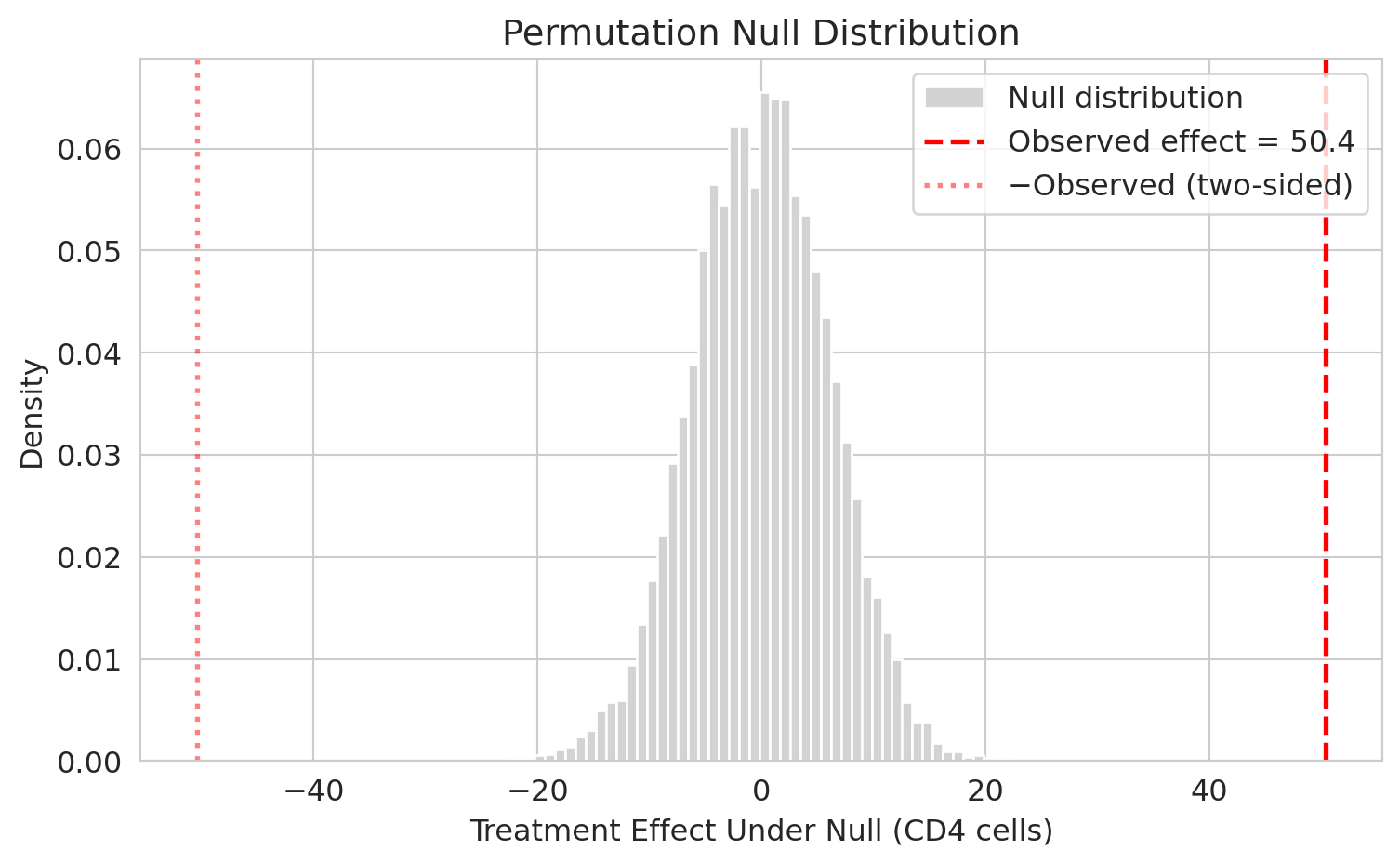
The red dashed line marks the observed effect of $+50.4$ CD4 cells. The picture answers the decision question: *if the drug did nothing, how often would shuffling alone produce an effect this far from zero?* Not one of the 10,000 permutations lands anywhere near $\pm 50$ — the observed effect sits in a region the null distribution never visits. That is what a very small p-value looks like. (Sanity check on your sketch: with ~1,000 patients per arm, the null distribution is much tighter than first-timers guess.) A drug that dramatically *hurt* patients would be just as noteworthy as one that dramatically helped, so we also mark the symmetric cutoff at $-50.4$ (red dotted line); the p-value below counts fake effects at least this far from zero in either direction.
## The p-value
:::{.callout-important}
## Definition: p-value
The probability of observing a result at least as extreme as what you got, assuming the null hypothesis is true.
:::
We compute a **two-sided** p-value: count permutations whose test statistic is at least as far from zero as the observed effect, in either direction. (We add $+1$ to numerator and denominator so a finite simulation can't report exactly 0; see Going deeper below.)
```{python}
# Count how many permutations produced an effect as extreme as observed
# Use absolute values for two-sided test
n_extreme = np.sum(np.abs(perm_effects) >= np.abs(observed_effect))

# Conservative estimator: (n_extreme + 1) / (n_perms + 1)
# This avoids reporting p = 0 exactly (Phipson & Smyth, 2010)
p_value = (n_extreme + 1) / (n_perms + 1)

print(f"Permutations with |effect| >= |{observed_effect:.1f}|: {n_extreme}")
print(f"p-value: {p_value:.4f}")
```
Across 10,000 shufflings, **zero** produced an effect as large as observed; the $+1$ correction is the only reason the value isn't exactly 0. The data are extremely surprising under the null of no effect — strong evidence the drug works.
### What the p-value is
The p-value is **a measure of surprise under the null**: a probability statement about the data, conditioned on $H_0$ being true. Three implications follow from that one fact.
- **It assumes the null.** A small p-value says *if there were no effect*, the data would be unlikely.
- **It is continuous evidence, not a verdict.** A p-value of $10^{-4}$ is far stronger evidence than $0.04$, even though both are "below 0.05."
- **It is computed from the observed data alone.** Replication, mechanism, and prior plausibility are not in the formula.
### What the p-value is not
The p-value is one of the most misinterpreted quantities in statistics. The cleanest way to learn the traps is to walk into one.
:::{.callout-tip}
## Think about it
A skeptic says: "A p-value of 0.0001 means there's only a 0.01% chance the drug doesn't work." Is the skeptic right? Think through your answer before reading on.
<details><summary>Answer</summary>
No — the skeptic flipped the conditional. The p-value is $P(\text{data this extreme} \mid H_0 \text{ true})$; the skeptic is claiming $P(H_0 \text{ true} \mid \text{data})$. "P(umbrella | raining)" is not "P(raining | umbrella)." Going from one to the other requires Bayes' theorem and a prior on $H_0$ — neither of which the p-value uses.
</details>
:::
:::{.callout-warning}
## Three traps
1. **A p-value is NOT the probability that $H_0$ is true.** That is the skeptic's flipped-conditional error above.
2. **A p-value is NOT the probability the result will replicate.** Replication depends on power, sampling variability, and whether the effect actually exists — none of which a single p-value pins down.
3. **p = 0.049 and p = 0.051 are not meaningfully different.** The 0.05 threshold is a convention, not a phase transition. Report the number; resist binary verdicts.
:::
:::{.callout-note collapse="true"}
## Going deeper: why add 1?
A p-value of exactly zero would claim infinite evidence against the null — a claim no finite simulation can support. Adding 1 to the numerator counts the observed data as one of the permutations (the identity permutation is always a permutation; under the null it is equidistributed with every other). Adding 1 to the denominator adjusts the total accordingly. The resulting estimator is **conservative**: under the null, its expected value is at least the nominal false-positive rate, so the finite-simulation p-value still controls false positives at the nominal level (Phipson & Smyth, 2010). The small upward bias shrinks as $n_{\text{perms}}$ grows.
:::
## From randomization to observation: do NBA refs favor the home team?
ACTG 175 was a *randomized* clinical trial: patients were assigned to arms by coin flip. That randomization is what licenses the causal interpretation — reject the null, and we conclude the drug *caused* the effect. Most real data is not like that. With observational groups, the permutation mechanics are identical, but the conclusions narrow sharply: a significant test tells us the two groups differ, not *why*.
To see that difference in action, we switch to a folk hypothesis NBA fans argue about endlessly: **referees favor the home team**. Moskowitz and Wertheim made the popular case in *Scorecasting* (2011), documenting systematic pro-home biases across sports — called strikes in baseball, stoppage time in soccer, foul calls in basketball — and arguing these referee effects explain most of home-court advantage. If they're right, one place it should show up is **personal foul** counts: home teams should be called for fewer of them than visiting opponents. Three NBA regular seasons (2021-22 through 2023-24) give us the data to test it.
**The null has the same shape as before**: home-team and away-team foul counts come from the same distribution. If that is true, the home/away label carries no information about fouls, and shuffling produces valid null draws.
**What's different is the interpretation of rejecting it.** No referees were randomly assigned to be home- or away-biased, and no games were randomly assigned home-or-away. Rejecting the null would tell us the two foul-count distributions differ — but it would *not* tell us *why*. Referee bias is one possible story, but other mechanisms ride along with the home/away label; the next Think About It asks you to generate some before we run the test.
:::{.callout-tip}
## Think about it
Suppose the permutation test finds that home teams are called for fewer fouls than away teams. Referee bias is the folk-theory explanation — but it is only one possibility. What are at least three **alternative** mechanisms, confounded with the home/away label, that could produce the same gap? Write them down before reading on.
<details><summary>Some alternatives</summary>
(a) **Fatigue and travel.** The visiting team has almost always traveled more recently. Tired defenders reach in instead of sliding their feet, and reaching fouls get called. (b) **Scheduling.** Back-to-backs (two games on consecutive nights) hit the visiting side of a given date more often than the home side over a season; compound that with (a). (c) **Defensive style.** A team may play more aggressively at home (leaning on crowd pressure) or less aggressively (feeling secure). Either asymmetry feeds into foul counts. (d) **Familiarity.** The home team knows its own sightlines, rim stiffness, and the exact location of the sideline — visiting players misposition and collide. (e) **Referee bias.** The hypothesis we started with. A permutation test cannot decompose which of (a)-(e) produces the gap; the 2020 "bubble" playoffs in Orlando — every game on a neutral court with no fans — are the closest thing we have to a natural experiment that strips many of these confounds away.
</details>
:::
The raw file is player-level: one row per player per game. We aggregate fouls to team-game totals by summing within each (game, team) pair, then label each team-game as home or away using the `MATCHUP` string (`"LAL vs. GSW"` = home, `"LAL @ GSW"` = away).
```{python}
logs = pd.read_csv(f'{DATA_DIR}/nba/nba_game_logs_2022_2024.csv',
                   usecols=['GAME_ID', 'TEAM_ABBREVIATION', 'MATCHUP', 'PF'])

team_game = (logs.groupby(['GAME_ID', 'TEAM_ABBREVIATION', 'MATCHUP'], as_index=False)
                 ['PF'].sum())
team_game['home'] = team_game['MATCHUP'].str.contains('vs.')

home_pf = team_game[team_game['home']]['PF'].values
away_pf = team_game[~team_game['home']]['PF'].values

obs_diff_nba = home_pf.mean() - away_pf.mean()
print(f"Home: {home_pf.mean():.2f} fouls per game   (n = {len(home_pf)})")
print(f"Away: {away_pf.mean():.2f} fouls per game   (n = {len(away_pf)})")
print(f"Observed difference (home − away): {obs_diff_nba:+.3f} fouls per game")
```
Home teams are called for about 0.18 fewer fouls per game. That is small against a typical 19-to-20-foul game, but over thousands of team-games the question sharpens: is the gap distinguishable from chance under the null? Recall the `permutation_diff_of_means` helper from the ACTG analysis — the machinery is identical here. Shuffle home/away labels, recompute the difference, repeat.
```{python}
all_pf = np.concatenate([home_pf, away_pf])
n_home = len(home_pf)

perm_diffs = np.array([
    permutation_diff_of_means(all_pf, n_home)
    for _ in range(10_000)
])

n_extreme_nba = np.sum(np.abs(perm_diffs) >= np.abs(obs_diff_nba))
p_value_nba = (n_extreme_nba + 1) / (len(perm_diffs) + 1)
print(f"Permutation p-value (two-sided): {p_value_nba:.4f}")
```
```{python}
fig, ax = plt.subplots(figsize=(8, 5))
counts, edges, _ = ax.hist(perm_diffs, bins=50, density=True,
color='lightgray', edgecolor='white',
label='Null distribution')
# Select bins by edges so partial tail bins get shaded.
in_right_tail = edges[:-1] >= abs(obs_diff_nba)
in_left_tail = edges[1:] <= -abs(obs_diff_nba)
in_tail = in_right_tail | in_left_tail
if in_tail.any():
ax.bar(edges[:-1][in_tail], counts[in_tail],
width=edges[1] - edges[0], align='edge',
color='#d7263d', alpha=0.7,
label='"At least as extreme" (two-sided)')
ax.axvline(obs_diff_nba, color='#d7263d', lw=2, ls='--',
label=f'Observed diff = {obs_diff_nba:+.3f} fouls')
ax.axvline(-obs_diff_nba, color='#d7263d', lw=2, ls=':', alpha=1.0,
label='−Observed (reflected cutoff)')
ax.set_xlabel('Difference in mean personal fouls: home − away')
ax.set_ylabel('Density')
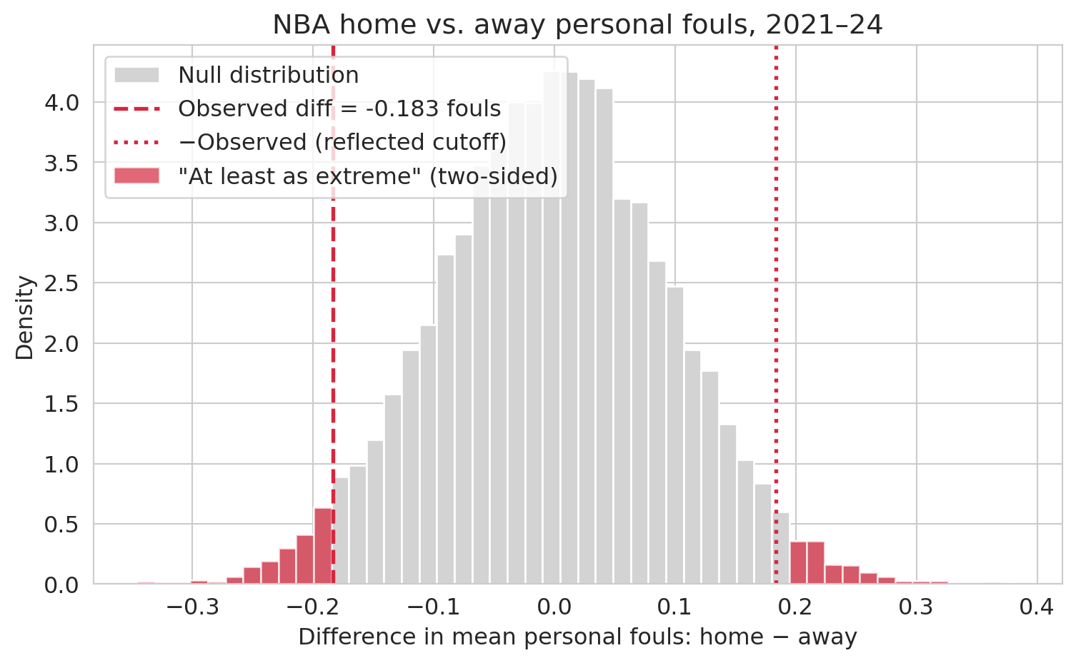
ax.set_title('NBA home vs. away personal fouls, 2021–24')
ax.legend(loc='upper left')
plt.tight_layout()
plt.show()
```
A very different picture from ACTG. Shuffled differences under the null wander up to about $\pm 0.3$ fouls per game, so the observed gap of $-0.18$ sits **at the edge of the null distribution, not outside it**. About 5% of permutations produce a difference at least as extreme — the p-value lands right at the conventional significance threshold $\alpha = 0.05$ (the cutoff below which a result is traditionally called "statistically significant"; we will use $\alpha$ for this threshold throughout). The data are *marginally* suggestive of a home-away difference, not decisive.
**The contrast with ACTG 175 is the point.** There, zero of 10,000 permutations reached the observed effect (p ≈ 0.0001) — the observed lived in a place the null never visits. Here, about 500 of 10,000 do, and we land near $\alpha = 0.05$. The useful contrast is **overwhelming evidence (ACTG, p ≈ 10⁻⁴) vs marginal evidence (fouls, p ≈ 0.05)**: report the number, not a yes/no.
And even if the data *did* convince us the groups differ, the observational setup still blocks the leap from "home teams are called for fewer fouls" to "refs favor the home team." Any of the mechanisms the Think About It asked you to generate could produce the gap on its own. (We return to association vs. causation in [Chapter 18](lec18-causal-inference-1.qmd).)
## One-sided vs two-sided tests
So far we've counted permutations extreme in *either* direction. That is the right default when effects in both directions matter — a harmful drug and a helpful one. But sometimes the scientific question is inherently one-directional. We motivated the NBA analysis with a directional folk hypothesis: **home teams get called for *fewer* fouls**. "Home foul count is *lower* than away" is narrower than "the two foul counts differ," and the narrower question calls for a **one-sided test**.
Let's compute both p-values on the same NBA permutation distribution and compare.
```{python}
# Two-sided: |fake diff| at least as large as |observed diff|
two_sided = (np.sum(np.abs(perm_diffs) >= np.abs(obs_diff_nba)) + 1) / (len(perm_diffs) + 1)

# One-sided (lower tail): fake diff as negative as observed or more so
# Pre-registered hypothesis: home teams commit fewer fouls, so home − away < 0.
one_sided = (np.sum(perm_diffs <= obs_diff_nba) + 1) / (len(perm_diffs) + 1)

print(f"Two-sided p-value:  {two_sided:.4f}")
print(f"One-sided p-value:  {one_sided:.4f}  (hypothesis: home < away)")
```
The one-sided number is about half the two-sided number, as the math predicts for an (approximately) symmetric null. What is striking is what this does to the verdict at the conventional threshold $\alpha = 0.05$: **the two-sided test fails to reject, and the one-sided test rejects**. Same data, different conclusion, driven entirely by an analytic choice.
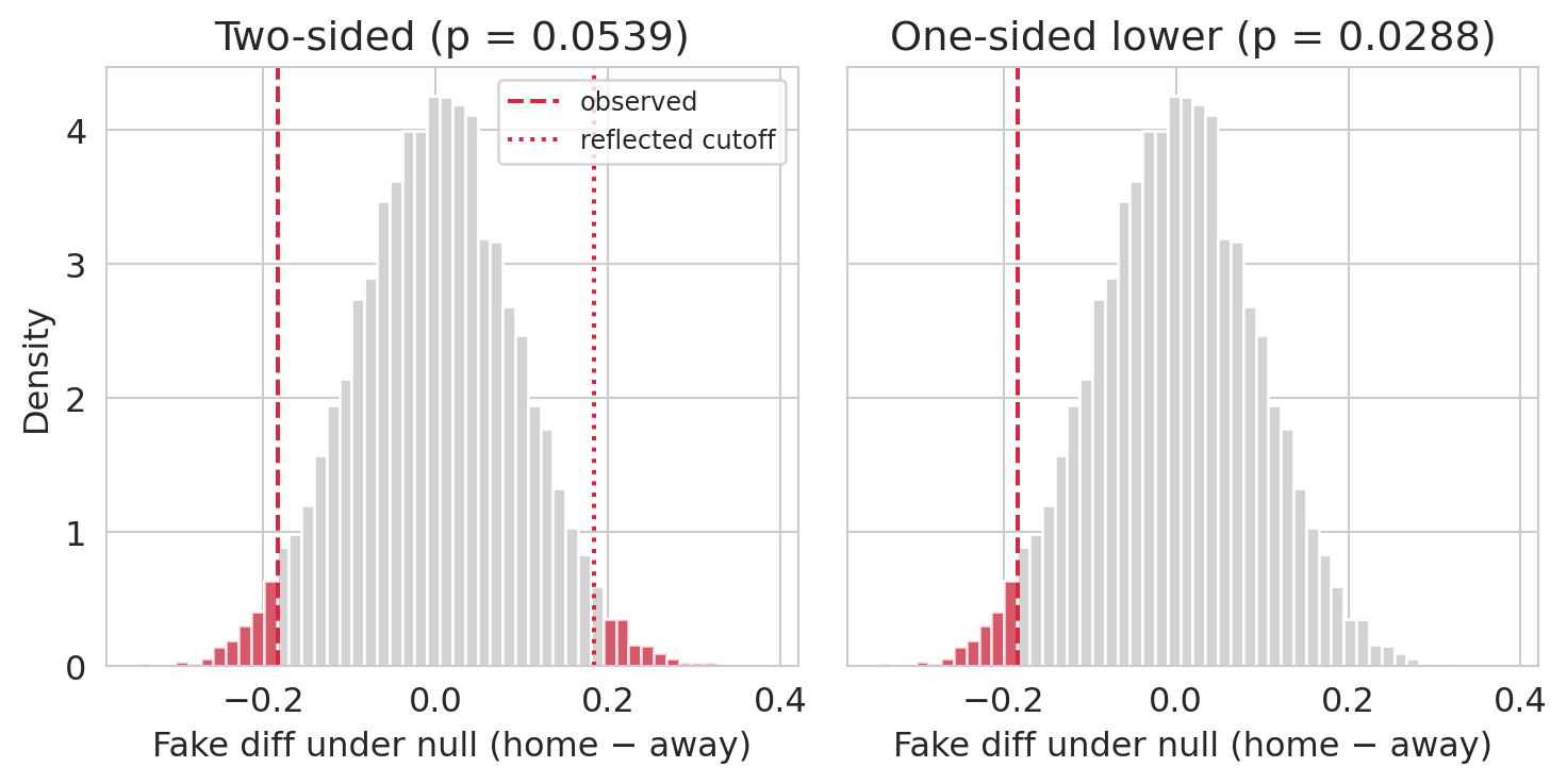
That is exactly why the direction has to be chosen *before* seeing the data. If the study's pre-registered protocol said "we expect home teams to get called for fewer fouls, test one-sided," the one-sided p-value is honest. If the analyst looked at the data, noticed that home foul counts were lower, and *then* declared the test one-sided, the one-sided p-value is a factor-of-two free lunch — the rate of falsely rejecting a true null is actually $2\alpha$, not $\alpha$. The picture below makes the counting rule visible on the same null distribution we already built.
```{python}
#| fig-cap: "Same null distribution, same observed statistic, two counting rules. Left — two-sided: both tails count. Right — one-sided (lower): only the tail of the hypothesized direction counts."
fig, axes = plt.subplots(1, 2, figsize=(8, 4), sharey=True)

# Left panel: two-sided counting rule
ax = axes[0]
counts, edges, _ = ax.hist(perm_diffs, bins=50, density=True,
                           color='lightgray', edgecolor='white')
# Select bins whose right edge crosses the positive cutoff OR whose
# left edge crosses the negative cutoff — uses edges (not centers) so
# partial tail bins aren't dropped.
in_right_tail = edges[:-1] >= abs(obs_diff_nba)
in_left_tail  = edges[1:]  <= -abs(obs_diff_nba)
in_tail = in_right_tail | in_left_tail
ax.bar(edges[:-1][in_tail], counts[in_tail],
       width=edges[1] - edges[0], align='edge',
       color='#d7263d', alpha=0.7)
ax.axvline( obs_diff_nba, color='#d7263d', lw=1.5, ls='--', label='observed')
ax.axvline(-obs_diff_nba, color='#d7263d', lw=1.5, ls=':', alpha=1.0,
           label='reflected cutoff')
ax.set_title(f'Two-sided (p = {two_sided:.4f})')
ax.set_xlabel('Fake diff under null (home − away)')
ax.set_ylabel('Density')
ax.legend(loc='upper right', fontsize=9)

# Right panel: one-sided (lower) counting rule
ax = axes[1]
counts, edges, _ = ax.hist(perm_diffs, bins=50, density=True,
                           color='lightgray', edgecolor='white')
# Select bins whose right edge is below the observed statistic.
in_tail = edges[1:] <= obs_diff_nba
ax.bar(edges[:-1][in_tail], counts[in_tail],
       width=edges[1] - edges[0], align='edge',
       color='#d7263d', alpha=0.7)
ax.axvline(obs_diff_nba, color='#d7263d', lw=1.5, ls='--', label='observed')
ax.set_title(f'One-sided lower (p = {one_sided:.4f})')
ax.set_xlabel('Fake diff under null (home − away)')

plt.tight_layout()
plt.show()
```
:::{.callout-important}
## Definition: One-sided and two-sided tests
A **two-sided test** counts permutations extreme in **either direction**: $|T_{\text{perm}}| \ge |T_{\text{obs}}|$. Use when effects in either direction would be noteworthy.
A **one-sided test** counts permutations in **one direction only**: $T_{\text{perm}} \ge T_{\text{obs}}$ (or $\le$, depending on the alternative). Use when only one direction is of scientific or practical interest — and **only when the direction was chosen before seeing the data.**
:::
When the null distribution is symmetric and continuous, the two-sided p-value is roughly double the one-sided. So "going one-sided" roughly halves your p-value — which is why the direction must be chosen *before* looking at the data. Picking the tail after seeing which way the observed statistic fell inflates the false-positive rate (what [Chapter 10](lec10-hypothesis-testing.qmd) will call the **Type I error rate**): a test nominally at $\alpha = 0.05$ rejects at rate $\approx 0.10$ under the null.
:::{.callout-note}
## A high-profile example: Deflategate
At halftime of the 2015 AFC Championship game, NFL officials measured the air pressure in the game footballs. The Patriots' balls came in below the legal minimum; the Colts' did not. Cooling physics explains *some* pressure drop — both teams played in the same cold weather on the same field — but the accusation was **directional**: the Patriots' balls had dropped *more* than the Colts', and by more than cooling alone could account for.
A Patriots ball that dropped *less* than the Colts' would have exonerated them, not indicted them. Only one direction counts as damaging — which is exactly what a one-sided test encodes.
:::
:::{.callout-tip}
## Think about it: pick the test
For each scenario, **state the null hypothesis precisely** in plain language and pick one-sided or two-sided. The phrasing matters: "the new curriculum doesn't *increase* scores" is a different null from "the new curriculum doesn't *change* scores," and they pick out different tests. For each answer, ask: *what decision rides on the result, and would a result in the other direction change it?*
1. A biotech company is running a Phase III trial of a new cholesterol drug, hoping it lowers LDL relative to standard care. The team must declare the test type before the trial begins.
2. A factory ships widgets under a contract that specifies a *minimum* mean weight: shipments below spec incur penalties; shipments above spec do not (heavy shipments just give the buyer extra product). The factory tests weekly samples to confirm compliance.
3. A school district rolled out a new math curriculum last year. They need to decide whether to keep it next year, roll back to the previous curriculum, or revise.
4. An airline is piloting a new boarding procedure on 50 flights to learn how it affects average boarding time.
<details><summary>Answers</summary>
(1) **Two-sided — a trap.** Null: $\mu_{\text{new}} = \mu_{\text{control}}$ (the drug doesn't *change* LDL). It is tempting to go one-sided since the team *hopes* LDL drops — but a drug that *raises* LDL is a safety signal, and that result would absolutely change the launch decision. Hoping for a direction is not the same as only one direction mattering.
<details><summary>Aside: what the FDA actually does</summary>
In real practice, FDA Phase III efficacy trials sometimes use a one-sided test at $\alpha = 0.025$ — which is equivalent in decision-theoretic terms to a two-sided test at $\alpha = 0.05$. The one-sidedness there is a regulatory convention paired with a separate safety-monitoring process, not a free halving of the p-value.
</details>
(2) **One-sided.** Null: $\mu \ge w_{\min}$ (the shipment meets the contract minimum); alternative: $\mu < w_{\min}$. The contract penalizes only under-weight shipments — over-weight is logically exculpatory, not noteworthy. The direction is fixed by the contract, not by the data. Same structure as Deflategate.
(3) **Two-sided.** Null: $\mu_{\text{new}} = \mu_{\text{old}}$ (the new curriculum doesn't *change* scores). The right framing is "no change," not "no increase": scores that *drop* drive the rollback decision, so the test has to be able to detect them. A one-sided "doesn't increase" null would silently treat a score drop as just another way to fail to detect an improvement, discarding evidence the district would act on.
(4) **Two-sided.** Null: $\mu_{\text{new}} = \mu_{\text{old}}$ (the new procedure doesn't change average boarding time). A slower procedure matters to operations as much as a faster one does.
Notice: three of four were two-sided, and the "trap" scenario (biotech) was too. One-sided tests are rare outside contract-compliance or tamper-detection contexts. Reserve them for cases where the other direction is *logically* irrelevant (not merely undesired), and pre-register the choice before looking at the data.
</details>
:::
Pulling the four scenarios together:
:::{.callout-warning}
## Prefer two-sided by default
If you are not sure which one to use, use a two-sided test. It is the honest default. A one-sided test is justified only when effects in the other direction are genuinely uninteresting or impossible — and that judgment must be pre-registered, not chosen after seeing which way the data pointed.
:::
## Bootstrap vs permutation: when to use which
These two simulation-based tools answer different questions:
| | Bootstrap | Permutation test |
|---|---|---|
| **Question** | How precise is my estimate? | Is the effect real? |
| **Produces** | Confidence interval | p-value |
| **Null hypothesis** | Not needed | Required |
| **Key assumption** | i.i.d. sample | Exchangeability under null |
| **Best for** | Any statistic | Comparing groups |
| **Resampling method** | With replacement, **within each group** separately | Without replacement, shuffling labels **across groups** |
**Bootstrap = precision. Permutation = significance. Use both.**
:::{.callout-tip}
## Think about it
Your bootstrap 95% CI for a treatment effect is [15, 85] — it excludes zero. Without computing anything, do you expect the permutation p-value to be above or below 0.05? Why?
<details><summary>Answer</summary>
Below 0.05. A 95% CI is built to contain the parameter values the data are *consistent* with at the 5% level. If zero is outside the CI, the data have ruled out "effect = 0" at that level — which is exactly what a two-sided test at $\alpha = 0.05$ reports. [Chapter 10](lec10-hypothesis-testing.qmd) makes this correspondence precise.
</details>
:::
The agreement we just derived — bootstrap CI and permutation p-value pointing at the same answer — is not a coincidence; [Chapter 10](lec10-hypothesis-testing.qmd) makes the link precise. For now the takeaway is practical: **if you already have a CI from Chapter 8, you have most of what a test would tell you**.
:::{.callout-note collapse="true"}
## Going deeper: the t-test as the parametric analog
Just as the bootstrap has a normal-approximation analog (the CLT-based CI from [Chapter 8](lec08-sampling.qmd)), the permutation test has one too: the **two-sample t-test**. The t-test assumes each group's mean is approximately normal (guaranteed by the CLT for large samples with finite variance) and computes a p-value from a t-distribution. [Chapter 10](lec10-hypothesis-testing.qmd) formalizes it as **Welch's t-test** and works through the design-based assumptions in detail; here we just check that the parametric analog and the permutation test agree on ACTG 175:
```{python}
t_stat, t_pvalue = stats.ttest_ind(treatment, control)
print(f"Two-sample t-test p-value: {t_pvalue:.3e}")
print(f"Permutation p-value:       {p_value:.4f}")
```
The t-test p-value is astronomically small — same conclusion as the permutation test, whose 0.0001 is the **simulation floor**: the true tail probability is even smaller, but a finite simulation can't see below $1/(m+1)$. The permutation test is distribution-free (it only needs exchangeability under the null) but requires simulation; the t-test is fast but assumes the CLT has kicked in. For large samples like these, either is fine; for small or heavily skewed samples, prefer the permutation test.
:::
## Key takeaways
- **Permutation test**: shuffle group labels to simulate the null hypothesis, then measure how often chance produces something as extreme as what you observed.
- **The p-value** measures surprise under the null — it is NOT the probability the null is true.
- Permutation tests work for comparing groups **without distributional assumptions** — they only require exchangeability under the null (which random assignment guarantees).
- **Two-sided by default.** A one-sided test is appropriate only when only one direction is of interest, and the direction is chosen *before* looking at the data.
- **Random assignment licenses causal claims.** Without it (NBA home/away), a significant permutation test shows the groups differ but cannot decompose *why*.
- **Overwhelming vs marginal evidence.** A p-value of $10^{-4}$ (ACTG) and a p-value of $0.05$ (NBA fouls) are both "small," but they support very different statements. Report the number, not a yes/no verdict.
- **Bootstrap measures precision** (confidence interval); **permutation measures significance** (p-value). They agree on the same evidence — a 95% CI excluding zero and a p-value below 0.05 say the same thing — which [Chapter 10](lec10-hypothesis-testing.qmd) makes precise.
- **Next**: [Chapter 10](lec10-hypothesis-testing.qmd) formalizes hypothesis testing — $H_0$, $H_1$, $\alpha$, Type I/II errors, and power.
## Study guide
### Key ideas
- **Null hypothesis**: The default claim being tested — typically "there is no effect" or "no difference between groups."
- **Test statistic**: The quantity computed from the data to measure the effect (here, difference in means).
- **Permutation test**: A hypothesis test that builds the null distribution by shuffling group labels and recomputing the test statistic. Requires exchangeability under the null (e.g., random assignment).
- **Null distribution**: The distribution of a test statistic under the assumption that the null hypothesis is true.
- **p-value**: The fraction of permutation samples producing a test statistic as extreme as observed (in absolute value, for a two-sided test). Equivalently, the probability of data this extreme under the null.
- **Exchangeability**: The property that swapping labels between groups does not change the joint distribution under the null. Random assignment guarantees exchangeability.
- **Two-sided test**: A test that counts extreme values in both tails — effects large in absolute value. Use when effects in either direction are noteworthy; this is the honest default.
- **One-sided test**: A test that counts extreme values in one tail only. Appropriate when only one direction of effect is of interest and the direction is chosen *before* seeing the data. Contract compliance and tamper-detection settings are the classic use cases; Deflategate is a vivid one-sided story (only under-inflation, not over-inflation, could indict the Patriots).
- **Bootstrap vs. permutation**: Bootstrap resamples **within each group** (with replacement) to measure precision. Permutation shuffles labels **across groups** (without replacement) to test significance.
- **Association vs. causation**: a permutation test can detect that two groups differ. Whether that difference is *caused* by group membership depends on whether the labels were randomly assigned.
- **Simulation-based inference**: The umbrella term for methods that build reference distributions by resampling (bootstrap, permutation test) rather than deriving them from a closed-form formula.
:::{.callout-tip}
## Worked example: p-value by hand
A tiny null distribution: `{-6, -3, -1, 0, 1, 2, 4, 5, 5, 7}`. Observed statistic: **4**.
- Two-sided count: permutations with $|v| \ge 4$ → $\{-6, 5, 5, 7\}$ → 4 permutations.
- Two-sided p-value: $(4 + 1)/(10 + 1) = 5/11 \approx 0.455$.
- One-sided (upper) count: permutations with $v \ge 4$ → $\{5, 5, 7\}$ → 3 permutations.
- One-sided p-value: $(3 + 1)/(10 + 1) = 4/11 \approx 0.364$.
Factor of 2-ish relationship preserved (not exact because the null isn't symmetric about 0 and the $+1$ corrections aren't symmetric either).
:::
### Computational tools
- `np.random.permutation(data)` — shuffle an array (for permutation tests)
- `np.sum(np.abs(perm_effects) >= np.abs(observed))` — count extreme permutations
- `(n_extreme + 1) / (n_perms + 1)` — conservative p-value estimator (the +1 counts the observed data as one of the permutations, preventing p = 0 from finite simulation)
- `stats.ttest_ind(group1, group2)` — two-sample t-test (parametric analog; see Going deeper box)
### For the quiz
You are responsible for: the permutation test procedure, null distributions, p-value computation (given a null distribution), two-sided vs one-sided reasoning, when a permutation test is valid (exchangeability), and distinguishing bootstrap from permutation tests. You are NOT responsible for: exact exchangeability proofs or t-test derivations.