---
title: "Working with AI"
execute:
enabled: true
jupyter: python3
---
You've been using random forests since [Chapter 13](lec13-trees.qmd) — fitting them to Airbnb data, watching test error plateau as you grow the forest. Today you learn *why* they work. And you'll see what happens when you hand your data to an AI and say "analyze this."
By the end of today, you'll understand why knowing statistics makes you a *better* user of AI tools, not an obsolete one. You'll also open the black box on trees: how recursive splitting works, why bootstrap samples and feature subsets make trees decorrelated, and how gradient boosting connects back to the gradient descent you saw in [Chapter 7](lec07-classification.qmd). The chapter ends with a 15-question checklist for evaluating any analysis — the delivery of the promise from Chapter 1.
```{python}
import numpy as np
import pandas as pd
import matplotlib.pyplot as plt
import seaborn as sns
from scipy import stats
from sklearn.linear_model import LinearRegression
from sklearn.tree import DecisionTreeRegressor, plot_tree, export_text
from sklearn.ensemble import RandomForestRegressor, GradientBoostingRegressor
from sklearn.model_selection import cross_val_score, KFold
from sklearn.preprocessing import StandardScaler
from sklearn.pipeline import Pipeline
from sklearn.metrics import r2_score, mean_absolute_error
import warnings
warnings.filterwarnings('ignore')
sns.set_style('whitegrid')
plt.rcParams['figure.figsize'] = (7, 4.5)
plt.rcParams['font.size'] = 12

DATA_DIR = 'data'
```
## How trees and forests work
In [Chapter 13](lec13-trees.qmd), you built decision trees and random forests for prediction. Trees split data recursively to minimize prediction error; forests average many overfit trees, using bootstrap samples and feature subsets to decorrelate them so averaging reduces variance. Here we examine which features matter most.
```{python}
# Load College Scorecard data
scorecard = pd.read_csv(f'{DATA_DIR}/college-scorecard/scorecard.csv')

feature_cols = ['SAT_AVG', 'UGDS', 'PCTPELL', 'PCTFLOAN', 'RET_FT4',
                'C150_4_POOLED_SUPP', 'CONTROL']
target_col = 'MD_EARN_WNE_P10'

for col in feature_cols + [target_col]:
    scorecard[col] = pd.to_numeric(scorecard[col], errors='coerce')

model_data = scorecard[feature_cols + [target_col]].dropna()
print(f"Complete cases: {len(model_data)} out of {len(scorecard)} ({len(model_data)/len(scorecard):.1%})")
```
```{python}
earnings_features = model_data[feature_cols]
earnings_target = model_data[target_col]

forest = RandomForestRegressor(n_estimators=100, random_state=42)
forest.fit(earnings_features, earnings_target)
forest_cv = cross_val_score(forest, earnings_features, earnings_target, cv=5, scoring='r2')
```
```{python}
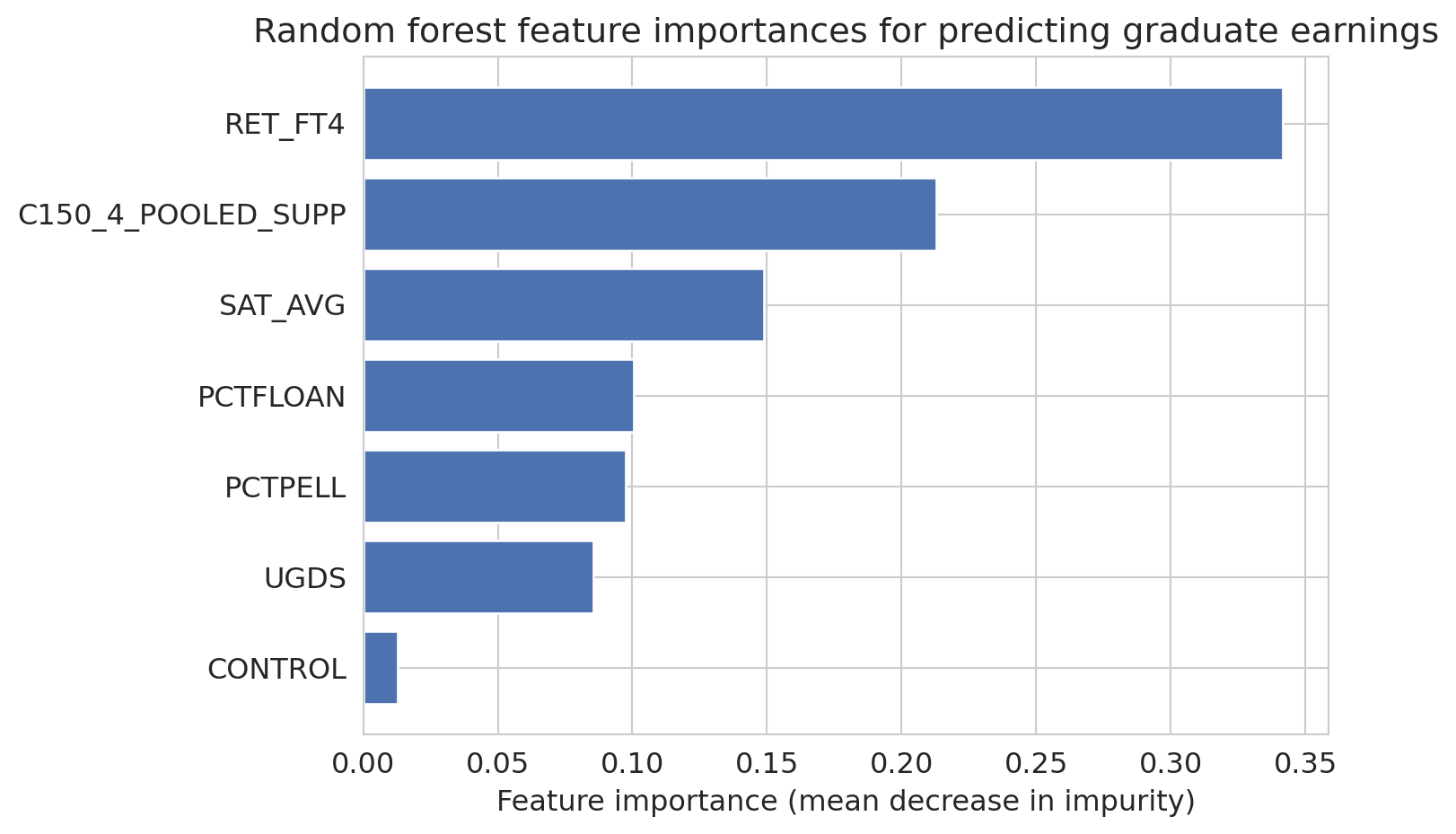
# Feature importances: one of the most practically useful RF outputs
importances = forest.feature_importances_
sorted_idx = np.argsort(importances)

fig, ax = plt.subplots(figsize=(8, 5))
ax.barh(np.array(feature_cols)[sorted_idx], importances[sorted_idx], color='#4C72B0')
ax.set_xlabel('Feature importance (mean decrease in impurity)')
ax.set_title('Random forest feature importances for predicting graduate earnings')
plt.tight_layout()
plt.show()
```
:::{.callout-tip}
## Think About It
Why does averaging many overfitting trees produce a good model? Hint: each tree overfits to *different* noise, given that it sees different bootstrap samples and different feature subsets.
:::
### What trees can do that linear regression can't
Three features of trees explain why they dominate tabular leaderboards. [Chapter 13](lec13-trees.qmd) introduced each; here we look at them through the lens of "what was Chapter 4's linear model missing?"
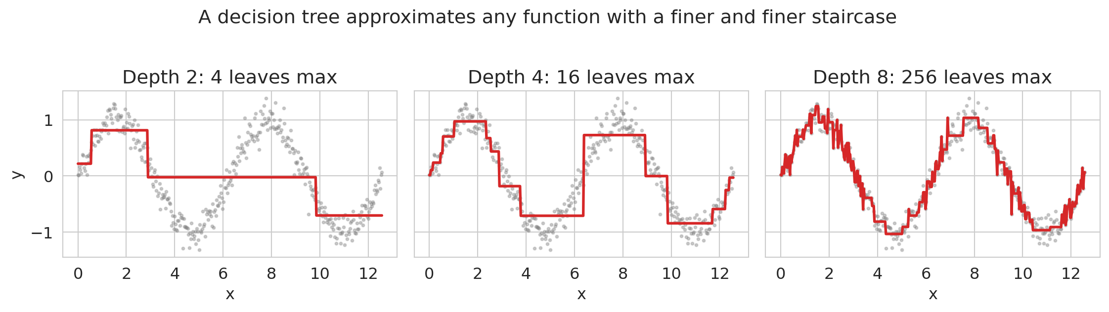
**Nonlinearities, for free.** A tree asks yes/no questions about feature values and predicts a constant in each resulting region. No $\beta x + \beta x^2 + \beta x^3 + \dots$, no manually designed interactions. The tree fits whatever shape the data requires — it just approximates it with a staircase. Let's make this concrete with a 1-D example.
```{python}
# Tree as a piecewise-constant function approximator
x_demo = np.linspace(0, 4*np.pi, 400)
y_demo = np.sin(x_demo) + 0.15 * np.random.default_rng(0).standard_normal(400)

fig, axes = plt.subplots(1, 3, figsize=(12, 3.2), sharey=True)
for ax, depth in zip(axes, [2, 4, 8]):
    tree = DecisionTreeRegressor(max_depth=depth, random_state=0)
    tree.fit(x_demo.reshape(-1, 1), y_demo)
    y_pred = tree.predict(x_demo.reshape(-1, 1))
    ax.scatter(x_demo, y_demo, s=4, alpha=0.35, color='gray')
    ax.plot(x_demo, y_pred, color='#d62728', lw=2)
    ax.set_title(f'Depth {depth}: {2**depth} leaves max')
    ax.set_xlabel('x')
axes[0].set_ylabel('y')
fig.suptitle('A decision tree approximates any function with a finer and finer staircase', y=1.02)
plt.tight_layout()
plt.show()
```
A depth-2 tree has up to 4 leaves and captures the broad strokes; depth-8 has up to 256 leaves and traces the sine curve closely. Increasing depth trades smoothness for expressiveness. Linear regression couldn't approximate this function at all without you first writing down `sin(x)` as a feature.
**Missing values handled natively.** In [Chapter 3](lec03-munging.qmd) we had to decide what to do with missing values before fitting any linear model. Trees can just add "is this value missing?" as another split direction. The two modern options:
- **Missingness Incorporated in Attributes (MIA).** At each split, the tree evaluates both options — sending missing rows left, or sending them right — and keeps whichever reduces loss more. This lets missingness itself carry signal when it's informative (e.g., income unreported because the respondent was unemployed). As of scikit-learn 1.4 (January 2024), this is the default behavior for `DecisionTreeRegressor`, `RandomForestRegressor`, and `HistGradientBoostingRegressor`: you can pass `NaN` directly and the tree learns a direction per node.
- **Surrogate splits.** Classical CART's fallback: when the primary split variable is missing for a row, use a correlated variable's threshold as a backup. R's `rpart` uses this; `sklearn` does not.
Both approaches matter because missingness is often **informative**: the fact that a variable is missing carries real signal (Van Ness, Bosschieter, Halpin-Gregorio, Udell 2023).^[Van Ness, M., Bosschieter, T. M., Halpin-Gregorio, R., & Udell, M. (2023). "The Missing Indicator Method: From Low to High Dimensions." KDD 2023.] For linear models, the standard fix is to add an explicit missingness-indicator column alongside an imputed value. For trees, MIA bakes the same idea into the split itself.
:::{.callout-note collapse="true"}
## Going deeper: pre-imputation with MissForest
Another option is to impute the missing values before fitting the model. **MissForest** (Stekhoven & Bühlmann 2012) is a popular method that uses random forests as the imputation engine itself: for each column with missing values, it fits an RF using the other columns as predictors, fills in the predictions, and iterates until the imputations stabilize. It handles mixed continuous/categorical data and uses the RF's out-of-bag error to self-assess, making it a strong default when you don't know what else to use. The downside is that pre-imputation discards information unless you also add an indicator column — which is why MIA-style methods that keep missingness as a live signal often win when missingness is informative.
:::
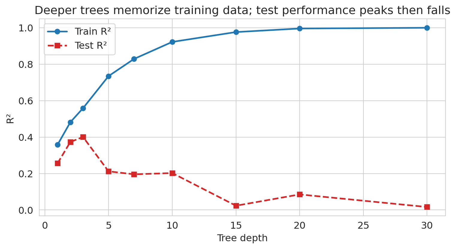
**Overfitting is controlled by depth.** A fully grown tree can achieve zero error on any training set — every row gets its own leaf. That's classic overfitting. Let's watch it happen on the College Scorecard data.
```{python}
# Train vs test error as tree depth grows: the classic overfitting curve
from sklearn.model_selection import train_test_split

X_depth = model_data[feature_cols].values
y_depth = model_data[target_col].values
X_tr, X_te, y_tr, y_te = train_test_split(X_depth, y_depth, test_size=0.3, random_state=42)

depths = [1, 2, 3, 5, 7, 10, 15, 20, 30]
train_r2 = []
test_r2 = []
for d in depths:
    t = DecisionTreeRegressor(max_depth=d, random_state=42).fit(X_tr, y_tr)
    train_r2.append(t.score(X_tr, y_tr))
    test_r2.append(t.score(X_te, y_te))

fig, ax = plt.subplots(figsize=(8, 4.5))
ax.plot(depths, train_r2, 'o-', color='#1f77b4', lw=2, label='Train R²')
ax.plot(depths, test_r2, 's--', color='#d62728', lw=2, label='Test R²')
ax.set_xlabel('Tree depth')
ax.set_ylabel('R²')
ax.set_title('Deeper trees memorize training data; test performance peaks then falls')
ax.legend()
plt.tight_layout()
plt.show()
```
Train R² climbs toward 1 as depth grows; test R² peaks around a moderate depth and then collapses as the tree starts fitting idiosyncratic training noise. This is the Chapter 6 overfitting story again, visible for a single learner. Random forests and gradient boosting exist in part to let *many* high-depth trees average away each other's idiosyncratic fits.
### Gradient boosting: learning from mistakes
There's another way to combine trees. Instead of growing them independently and averaging, **gradient boosting** grows them *sequentially*: each new tree is trained on the *errors* of the previous trees.
Each new tree fits the negative gradient (pseudo-residuals) of the loss. For squared loss, the negative gradient *is* the residual `y − ŷ` — so each tree literally trains on the previous ensemble's errors. Just as gradient descent ([Chapter 7](lec07-classification.qmd)) takes steps in parameter space, gradient boosting takes steps in *function space* by adding a tree that approximates the negative gradient. Each added tree nudges the ensemble's prediction a little closer to the truth.
```{python}
# Gradient boosting: sequential error correction
gboost = GradientBoostingRegressor(n_estimators=100, random_state=42)
gboost.fit(earnings_features, earnings_target)
gboost_cv = cross_val_score(gboost, earnings_features, earnings_target, cv=5, scoring='r2')

print(f"Random Forest:     CV R-sq = {forest_cv.mean():.3f}")
print(f"Gradient Boosting: CV R-sq = {gboost_cv.mean():.3f}")
print(f"\nGradient boosting often edges out random forests on tabular data.")
```
Now you know what's inside the black box. Let's see how AutoML uses these tools — and what it still can't do.
## The AutoML promise
:::{.callout-important}
## Definition: AutoML
**AutoML** (automated machine learning) takes this further: tools like auto-sklearn, H2O AutoML, and Google Vertex AI automatically try hundreds of model configurations — including trees, forests, gradient boosting, and others — and pick the best one. No feature engineering, no hyperparameter tuning.
:::
Under the hood, some AutoML systems also try additive models and splines — smooth nonlinear models that are more interpretable than random forests but more flexible than linear regression.
Let's simulate this with a "poor man's AutoML": try several models with cross-validation and pick the winner.
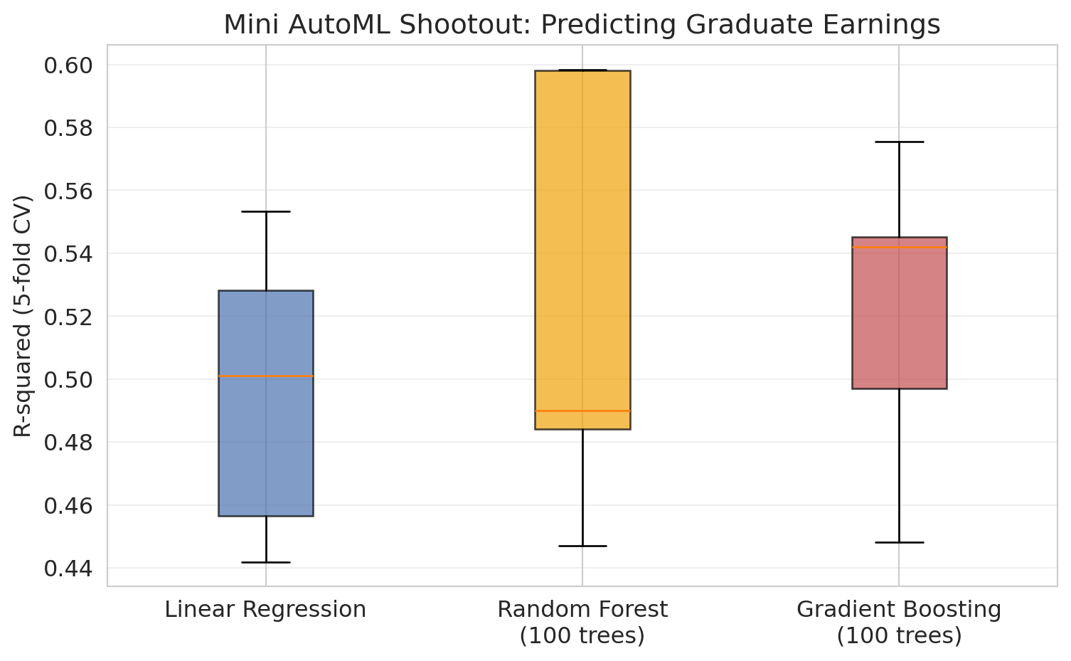
```{python}
# Poor man's AutoML: try 3 models, pick the best by 5-fold CV
# Use Pipeline to prevent data leakage (scaler only sees training folds)
kf = KFold(n_splits=5, shuffle=True, random_state=42)

models = {
    'Linear Regression': Pipeline([('scaler', StandardScaler()), ('model', LinearRegression())]),
    'Random Forest\n(100 trees)': RandomForestRegressor(n_estimators=100, random_state=42),
    'Gradient Boosting\n(100 trees)': GradientBoostingRegressor(n_estimators=100, random_state=42),
}

cv_results = {}
print(f"{'Model':<35} {'Mean R-sq':>10} {'Std':>8} {'Mean MAE':>10}")
print("=" * 68)
best_score = -np.inf
best_name = None

for name, model in models.items():
    features = model_data[feature_cols].values
    target = model_data[target_col].values
    r2_scores = cross_val_score(model, features, target, cv=kf, scoring='r2')
    mae_scores = -cross_val_score(model, features, target, cv=kf, scoring='neg_mean_absolute_error')
    cv_results[name] = r2_scores
    display_name = name.replace('\n', ' ')
    print(f"{display_name:<35} {r2_scores.mean():>10.3f} {r2_scores.std():>8.3f} {mae_scores.mean():>10.0f}")
    if r2_scores.mean() > best_score:
        best_score = r2_scores.mean()
        best_name = display_name

print(f"\nWinner: {best_name} (R-sq = {best_score:.3f})")
print("AutoML would do this with hundreds of models and fancier tuning.")
```
```{python}
# Visualize the CV results
fig, ax = plt.subplots(figsize=(8, 5))
bp = ax.boxplot([scores for scores in cv_results.values()],
                tick_labels=list(cv_results.keys()),
                patch_artist=True)
colors = ['#4C72B0', '#F0A30A', '#C44E52']
for patch, color in zip(bp['boxes'], colors):
    patch.set_facecolor(color)
    patch.set_alpha(0.7)
ax.set_ylabel('R-squared (5-fold CV)')
ax.set_title('Mini AutoML Shootout: Predicting Graduate Earnings')
ax.grid(axis='y', alpha=0.3)
plt.tight_layout()
plt.show()
```
Not bad! Random Forest edges out gradient boosting here. AutoML *works* — for the modeling step.
:::{.callout-tip}
## Think About It
Before we continue — what did AutoML NOT do here? What decisions did *we* make before any model was fit?
:::
## What AutoML can't do
Let's look at what got swept under the rug. What kinds of schools did we lose by requiring complete data?
```{python}
# What did we lose by dropping missing values?
print("Institutions with complete data vs. all institutions:")
print(f"  All institutions:    {len(scorecard):,}")
print(f"  With SAT_AVG:        {scorecard['SAT_AVG'].notna().sum():,}")
print(f"  With earnings data:  {pd.to_numeric(scorecard[target_col], errors='coerce').notna().sum():,}")
print(f"  Complete cases:      {len(model_data):,}")
```
```{python}
# What kinds of schools are we dropping?
scorecard_analysis = scorecard.copy()
scorecard_analysis['has_data'] = scorecard.index.isin(model_data.index)
control_labels = {1: 'Public', 2: 'Private nonprofit', 3: 'Private for-profit'}
scorecard_analysis['control_label'] = pd.to_numeric(scorecard_analysis['CONTROL'], errors='coerce').map(control_labels)

retention_data = []
print("Representation by institution type:")
for label in ['Public', 'Private nonprofit', 'Private for-profit']:
    total = (scorecard_analysis['control_label'] == label).sum()
    kept = ((scorecard_analysis['control_label'] == label) & scorecard_analysis['has_data']).sum()
    if total > 0:
        pct = kept / total
        print(f"  {label:<25s} {kept:>5d} / {total:>5d} ({pct:.0%} kept)")
        retention_data.append({'type': label, 'kept': kept, 'total': total, 'pct': pct})
```
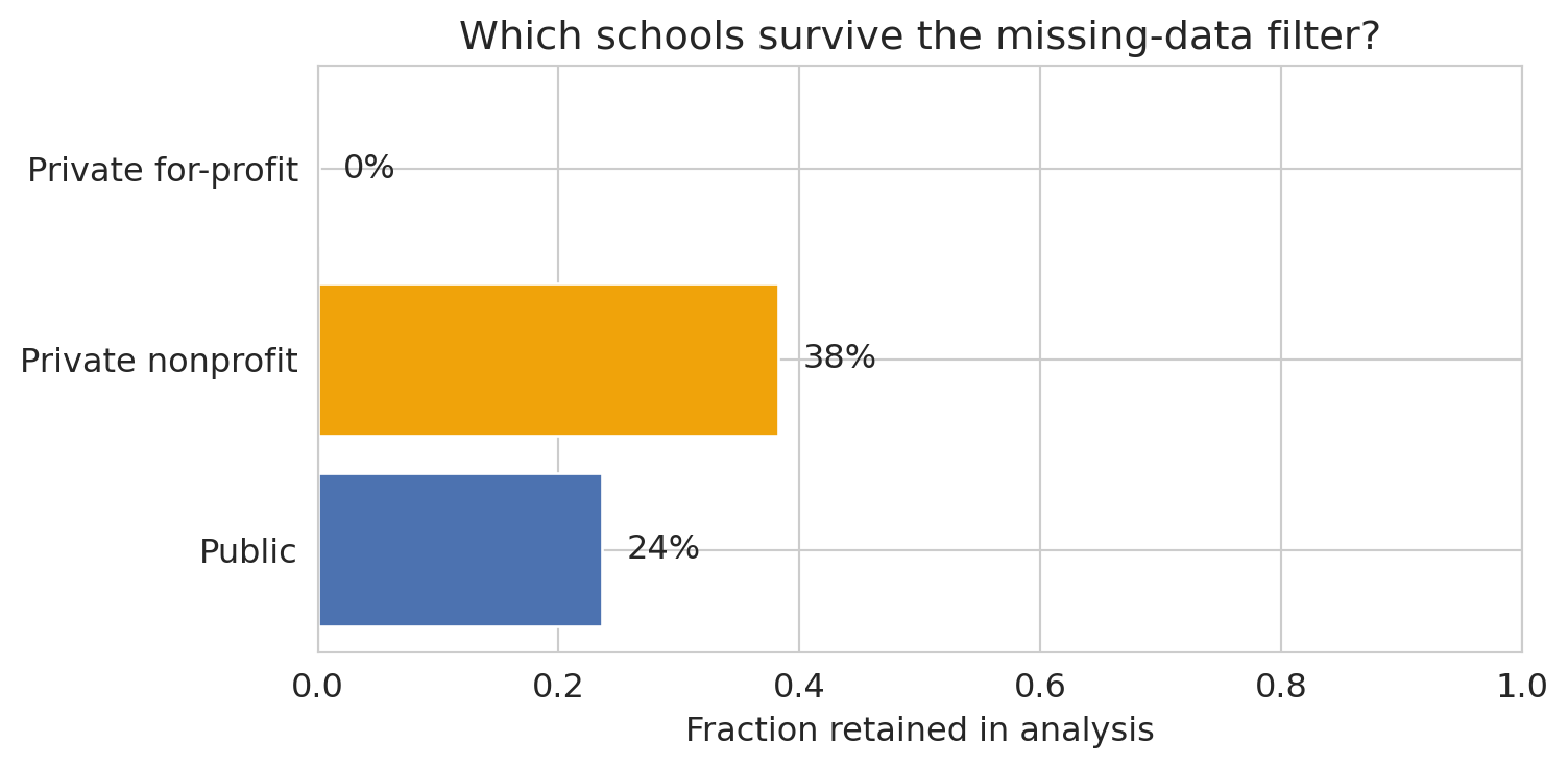
```{python}
# Visualize the selection bias
retention_df = pd.DataFrame(retention_data)
fig, ax = plt.subplots(figsize=(8, 4))
bars = ax.barh(retention_df['type'], retention_df['pct'], color=['#4C72B0', '#F0A30A', '#C44E52'])
ax.set_xlabel('Fraction retained in analysis')
ax.set_title('Which schools survive the missing-data filter?')
ax.set_xlim(0, 1)
for bar, row in zip(bars, retention_data):
    ax.text(bar.get_width() + 0.02, bar.get_y() + bar.get_height()/2,
            f"{row['pct']:.0%}", va='center')
plt.tight_layout()
plt.show()
```
This exclusion pattern is **selection bias** from [Chapter 3](lec03-munging.qmd). By requiring SAT scores, we've excluded community colleges, trade schools, and most for-profit institutions — precisely the schools where the relationship between institutional characteristics and earnings might be *different*.
AutoML optimized R-squared on the available data. It has no way to know the available data isn't representative.
## The LLM revolution
**Large Language Models** (**LLMs**) like ChatGPT, Claude, and Gemini go further than AutoML. LLMs can extract structured features from unstructured text (turning a free-form listing description into "has_wifi", "near_transit", "is_luxury"), and they can go further — you can say "analyze this dataset" in plain English and get working code, visualizations, and interpretations back.
Let's see what happens when we ask an LLM to analyze data. Below is the kind of code an LLM might produce — and it *looks* reasonable.
```{python}
# What an LLM might generate when asked:
# "Load the College Scorecard data and find what predicts higher earnings"
# (LLM-generated code tends to use short variable names like this)

# Step 1: Load data (LLM gets this right)
sc = pd.read_csv(f'{DATA_DIR}/college-scorecard/scorecard.csv')

# Step 2: "Clean" the data (LLM drops rows with any missing values)
numeric_cols = ['SAT_AVG', 'UGDS', 'PCTPELL', 'PCTFLOAN',
                'MD_EARN_WNE_P10', 'RET_FT4']
for col in numeric_cols:
    sc[col] = pd.to_numeric(sc[col], errors='coerce')

sc_clean = sc.dropna(subset=numeric_cols)
print(f"LLM 'cleaned' data: {len(sc_clean)} rows (dropped {len(sc) - len(sc_clean)})")
```
```{python}
# Step 3: Fit a regression (LLM picks a standard model)
X_llm = sc_clean[['SAT_AVG', 'UGDS', 'PCTPELL', 'PCTFLOAN', 'RET_FT4']]
y_llm = sc_clean['MD_EARN_WNE_P10']

model_llm = LinearRegression()
model_llm.fit(X_llm, y_llm)

# Notice: this is R-squared on the *training* data -- no cross-validation.
# From Lecture 6, we know this is optimistic.
print(f"R-squared: {model_llm.score(X_llm, y_llm):.3f}")
print("\nCoefficients:")
for feat, coef in zip(X_llm.columns, model_llm.coef_):
    print(f"  {feat:<20s} {coef:+.2f}")
print(f"\nLLM conclusion: 'SAT scores are the strongest predictor of earnings.'")
```
The code is clean. The R-squared is decent. The LLM would probably wrap this up with a confident interpretation: *"Higher SAT scores are associated with higher post-graduation earnings, suggesting that more selective institutions produce better-earning graduates."*
The code runs. The output looks reasonable. The descriptive association is real — but the causal interpretation slipped in by the second clause is wrong, and the analysis hides several other problems. Let's count them.
## Where LLMs fail
### Problem 1: Silent data loss
The LLM dropped most of the data without flagging it. The missingness here is not random — schools that don't report SAT scores are *systematically different* from those that do. This pattern is the **MNAR** (missing not at random) case from [Chapter 3](lec03-munging.qmd): schools with low SAT averages may be less likely to report them, and schools that don't require SATs (community colleges, trade schools) have no score to report at all.
```{python}
# The LLM didn't check what it dropped
print("What the LLM threw away:")
print(f"  Total institutions: {len(sc):,}")
print(f"  Kept: {len(sc_clean):,} ({len(sc_clean)/len(sc):.0%})")
print(f"  Dropped: {len(sc) - len(sc_clean):,} ({(len(sc) - len(sc_clean))/len(sc):.0%})")
```
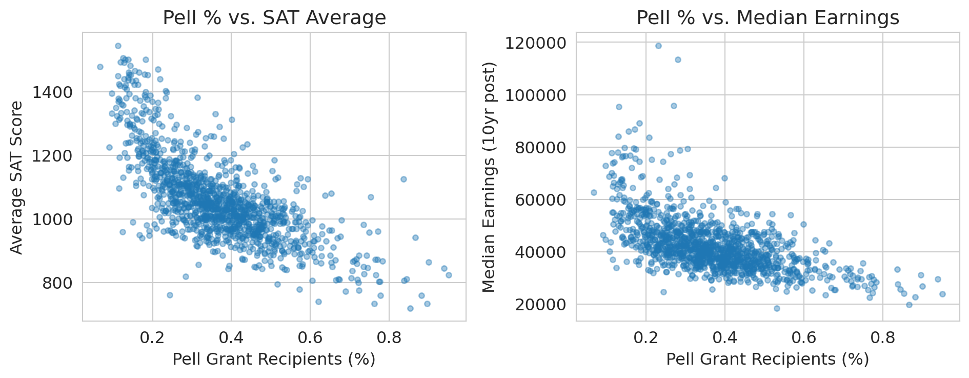
### Problem 2: Confusing correlation with causation
The LLM said SAT scores "predict" higher earnings. But does attending a higher-SAT school *cause* you to earn more? Or do higher-SAT schools simply admit students who would have earned more anyway?
This result reflects a **confounding** problem — the kind you saw in [Chapter 11](lec11-multiple-testing.qmd), formalized with DAGs in [Chapter 18](lec18-causal-inference-1.qmd). Family income, parental education, and geographic location all affect both SAT scores and earnings. The LLM has no way to distinguish confounded association from causal effect.
```{python}
# Show the confounding: Pell Grant % (a proxy for family income) correlates with both
fig, axes = plt.subplots(1, 2, figsize=(10, 4))

axes[0].scatter(sc_clean['PCTPELL'], sc_clean['SAT_AVG'], alpha=0.4, s=15)
axes[0].set_xlabel('Pell Grant Recipients (%)')
axes[0].set_ylabel('Average SAT Score')
axes[0].set_title('Pell % vs. SAT Average')

axes[1].scatter(sc_clean['PCTPELL'], sc_clean['MD_EARN_WNE_P10'], alpha=0.4, s=15)
axes[1].set_xlabel('Pell Grant Recipients (%)')
axes[1].set_ylabel('Median Earnings (10yr post)')
axes[1].set_title('Pell % vs. Median Earnings')

plt.tight_layout()
plt.show()

print("Family income (proxied by Pell %) drives BOTH SAT scores AND earnings.")
print("The SAT-earnings correlation is largely confounded by socioeconomic status.")
```
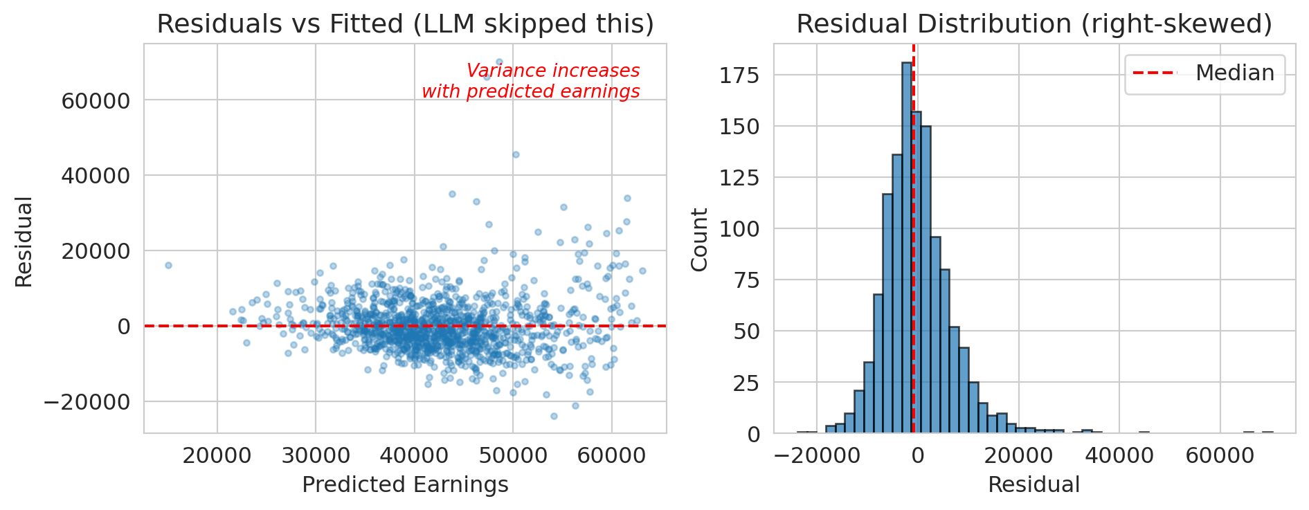
### Problem 3: No assumption checking
The LLM fit a linear regression without checking:
- Are the residuals approximately normal? (Probably not — earnings are right-skewed)
- Is the relationship actually linear?
- Are there influential outliers?
Recall from [Chapter 12](lec12-regression-inference.qmd): regression diagnostics aren't optional. They tell you whether your model's conclusions are trustworthy.
```{python}
# Quick residual check the LLM skipped
residuals = y_llm - model_llm.predict(X_llm)

fig, axes = plt.subplots(1, 2, figsize=(10, 4))

axes[0].scatter(model_llm.predict(X_llm), residuals, alpha=0.3, s=10)
axes[0].axhline(y=0, color='red', linestyle='--')
axes[0].set_xlabel('Predicted Earnings')
axes[0].set_ylabel('Residual')
axes[0].set_title('Residuals vs Fitted (LLM skipped this)')
# Annotate the fan shape
axes[0].annotate('Variance increases\nwith predicted earnings',
                 xy=(0.95, 0.95), xycoords='axes fraction',
                 ha='right', va='top', fontsize=10, color='red', style='italic')

axes[1].hist(residuals, bins=50, edgecolor='black', alpha=0.7)
axes[1].axvline(x=np.median(residuals), color='red', linestyle='--', label='Median')
axes[1].set_xlabel('Residual')
axes[1].set_ylabel('Count')
axes[1].set_title('Residual Distribution (right-skewed)')
axes[1].legend()

plt.tight_layout()
plt.show()

print("The residuals are right-skewed and show heteroscedasticity.")
print("The linear model's confidence intervals are unreliable.")
print("The LLM didn't check.")
```
### Problem 4: Hallucinated confidence
:::{.callout-warning}
## LLMs don't calibrate confidence
LLMs don't reliably calibrate their confidence. They may hedge on a simple calculation and then present a complex causal claim with the same confident tone. An LLM will:
- Report a p-value without checking if the test's assumptions are met
- Claim a result is "statistically significant" without considering multiple comparisons
- Make causal claims from observational data
:::
:::{.callout-tip}
## Think About It
Would you trust a colleague who never says "I don't know"? What would you do differently if you knew your analysis tool couldn't distinguish what it knows from what it's guessing?
:::
## LLM analysis vs. your analysis
Let's test this concretely. If you asked an LLM "Do NBA players perform better after rest?", here's roughly what it would do.
```{python}
# Load NBA data
nba = pd.read_csv(f'{DATA_DIR}/nba/nba_load_management.csv')
nba['GAME_DATE'] = pd.to_datetime(nba['GAME_DATE'])
print(f"NBA dataset: {len(nba):,} player-games")
print(f"Seasons: {nba['SEASON'].unique()}")
```
```{python}
# What an LLM would do: run a simple comparison
rested = nba[nba['REST_DAYS'] >= 3]['PTS']
not_rested = nba[nba['REST_DAYS'] <= 1]['PTS']

t_stat, p_value = stats.ttest_ind(rested, not_rested)

print("LLM's analysis: 'Do players score more when rested?'")
print(f"  Rested (3+ days):      {rested.mean():.1f} PPG (n={len(rested):,})")
print(f"  Not rested (0-1 days): {not_rested.mean():.1f} PPG (n={len(not_rested):,})")
print(f"  t-statistic: {t_stat:.2f}")
print(f"  p-value: {p_value:.2e}")
print()
if rested.mean() < not_rested.mean():
    print("Wait -- rested players score FEWER points?")
    print("The LLM would either report this surprising finding uncritically")
    print("or quietly reverse the groups to match its prior belief.")
```
Wait — rested players score *fewer* points? That's backwards from what you'd expect.
:::{.callout-tip}
## Think About It
Why might this be backwards? Think about *which* players tend to have many rest days, and *which* players play on back-to-backs. Take 30 seconds before reading on.
:::
This reversal is **Simpson's paradox** from [Chapter 11](lec11-multiple-testing.qmd). The aggregate comparison is *backwards*, given that rest is confounded with player quality:
- Bench players (low scorers) have more rest days — they don't play every game
- Stars (high scorers) play on back-to-backs — coaches need them
The LLM also used `ttest_ind` without noting that the same players appear many times — the observations within a player are correlated, violating the independence assumption.
The LLM doesn't know any of this. It would report the naive comparison and either:
1. Confidently claim rest *hurts* performance (wrong interpretation)
2. Hedge with "more analysis needed" (correct but unhelpful)
For the within-player analysis we switch from `PTS` to `GAME_SCORE`, a composite metric that accounts for rebounds, assists, turnovers, and efficiency — a better measure of overall performance than raw points.
```{python}
# What WE know to do: control for player identity
# Within-player comparison (from Lecture 11)
player_effects = []
players_tested = 0
significant_naive = 0

for player in nba['PLAYER_NAME'].unique():
    pdata = nba[nba['PLAYER_NAME'] == player]
    rested_p = pdata[pdata['REST_DAYS'] >= 3]['GAME_SCORE']
    tired_p = pdata[pdata['REST_DAYS'] <= 1]['GAME_SCORE']

    if len(rested_p) >= 10 and len(tired_p) >= 10:
        t, p = stats.ttest_ind(rested_p, tired_p)
        players_tested += 1
        if p < 0.05:
            significant_naive += 1
        player_effects.append({
            'player': player,
            'diff': rested_p.mean() - tired_p.mean(),
            'p_value': p
        })
```
```{python}
# Summarize the within-player results
effects_df = pd.DataFrame(player_effects)

print(f"Within-player analysis (the right way):")
print(f"  Players tested: {players_tested}")
print(f"  'Significant' at p<0.05: {significant_naive} ({significant_naive/players_tested:.1%})")
print(f"  Expected by chance (5%): {players_tested * 0.05:.0f}")
print()
print(f"  Mean effect (rested - tired): {effects_df['diff'].mean():+.2f} game score points")
print(f"  Median effect:                {effects_df['diff'].median():+.2f}")
```
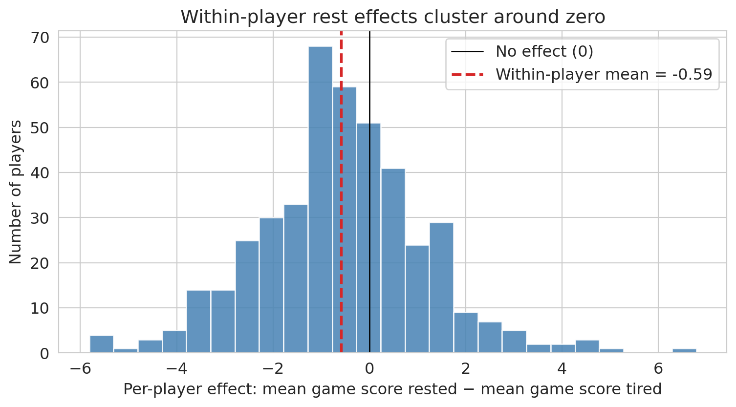
```{python}
# Visualize the distribution of per-player effects
fig, ax = plt.subplots(figsize=(8, 4.5))
ax.hist(effects_df['diff'], bins=25, color='steelblue', edgecolor='white', alpha=0.85)
ax.axvline(x=0, color='black', linestyle='-', linewidth=1, label='No effect (0)')
ax.axvline(x=effects_df['diff'].mean(), color='#d62728', linestyle='--', linewidth=2,
           label=f"Within-player mean = {effects_df['diff'].mean():+.2f}")
ax.set_xlabel('Per-player effect: mean game score rested − mean game score tired')
ax.set_ylabel('Number of players')
ax.set_title("Within-player rest effects cluster around zero")
ax.legend()
plt.tight_layout()
plt.show()
```
Each bar counts players whose rested-vs-tired difference falls in that bin. Most players sit near zero; a few outliers in each tail are roughly balanced, consistent with noise rather than a systematic rest effect. Compare this to the LLM's aggregate finding (rested players scoring *fewer* points) — once player identity is controlled for, that aggregate difference evaporates. The LLM's conclusion came entirely from the confounding between rest and player quality, not from any actual effect of rest on performance.
After controlling for player identity, the effect shrinks dramatically. Most "significant" per-player results are likely false positives from multiple testing ([Chapter 11](lec11-multiple-testing.qmd)). Even this within-player t-test is a simplification — a proper analysis would account for game context — but the point is that controlling for player identity greatly reduces the naive finding.
The LLM gave you a result in seconds. But it took 16 lectures of statistical training to know:
1. The aggregate comparison is confounded — this is Simpson's paradox ([Chapter 11](lec11-multiple-testing.qmd)), formalized causally in [Chapter 18](lec18-causal-inference-1.qmd)
2. You need within-player comparisons ([Chapter 11](lec11-multiple-testing.qmd))
3. Testing many players inflates false positives ([Chapter 11](lec11-multiple-testing.qmd))
4. The effect size is tiny even when "significant" ([Chapter 12](lec12-regression-inference.qmd))
The LLM got the *computation* right. It got the *thinking* wrong.
## What remains irreducibly human
AI tools are getting better fast. But some things remain fundamentally human:
**Asking the right question.** "What predicts earnings?" is a different question from "What *causes* higher earnings?" or "Which schools provide the most *value-added*?" The data can't tell you which question to ask.
:::{.callout-note}
## Tukey on asking the right question
"Far better an approximate answer to the right question, which is often vague, than an exact answer to the wrong question, which can always be made precise." — John Tukey
The LLM gave a precise answer to the wrong question. Tukey's warning, written long before LLMs existed, lands sharper today than ever.
:::
**Knowing the domain.** Why are for-profit schools missing SAT data? Why do bench players have more rest days? Why does AQI spike in August? Domain knowledge is the difference between a plausible-looking wrong answer and a correct one.
**Questioning assumptions.** Every statistical method makes assumptions. LLMs rarely check them. You now know to ask: Is this data representative? Is the relationship causal? Are the residuals well-behaved? Are we testing too many hypotheses?
**Understanding stakes and consequences.** A wrong prediction about air quality could mean people go outside during a hazardous event. A wrong conclusion about school quality could redirect billions in funding. The statistical method is the same; the consequences are not.
**Communicating uncertainty honestly.** LLMs project confidence. Good statisticians communicate uncertainty. "The model suggests X, but the confidence interval is wide and the data is missing for the most vulnerable populations" is more honest — and more useful — than "X."
:::{.callout-tip}
## Think About It
Which of these skills could an AI eventually learn? Which require human judgment that no amount of training data can replace?
:::
## A practical guide: using AI tools well
AI tools aren't going away. Here's how to use them as a *statistically literate* person:
| Use AI for... | But always check... |
|--------------|-------------------|
| Writing boilerplate code | Does it handle missing data correctly? |
| Quick EDA and visualization | Are the axes labeled? Is the scale misleading? |
| Trying multiple models | What data was dropped? What assumptions were violated? |
| Generating hypotheses | Is this correlation or causation? |
| Drafting reports | Are the uncertainty statements honest? |
The pattern: **let the AI draft, then apply your statistical judgment.** This principle is why you took the course.
This checklist is worth keeping — save it for when you use AI tools in your projects.
### Prompt decomposition: how to use AI effectively
Don't ask an LLM to "analyze this dataset." Break the task into smaller steps where you can verify each one:
1. **Load and inspect:** "Load this CSV and show me the first few rows, dtypes, and missing value counts."
2. **Check missingness:** "Which columns have missing values? Show me how missingness relates to other variables."
3. **Fit a model:** "Fit a linear regression of Y on X1, X2, X3. Show residual diagnostics."
4. **Check your work:** "What assumptions did this analysis make? What could go wrong?"
Each step gives you a checkpoint. If the LLM silently drops 84% of the data in step 1, you catch it before it propagates through the entire analysis.
:::{.callout-tip}
## Think About It
You've probably used AI tools for homework this quarter. Think of a time the AI gave you something that looked right but wasn't — or a time you caught a mistake the AI missed. What course concept helped you catch it?
:::
## Key takeaways
- **AutoML finds good models automatically**, but it can't choose the right question, check data quality, or interpret results in context. It optimizes math, not thinking.
- **LLMs write working code fast**, but they don't check assumptions, notice subtle data issues, or distinguish correlation from causation. They're confidently wrong about causal claims.
- **Trees, forests, and boosting** are the workhorse models behind most AutoML systems. Decision trees split data recursively; random forests average many trees to reduce variance; gradient boosting trains trees sequentially on residuals.
- **The biggest errors aren't computational.** They're conceptual: asking the wrong question, using biased data, confusing correlation with causation, ignoring multiple testing. These are human judgment calls.
- **AI tools are powerful assistants.** Use them for drafting code, trying models, and generating hypotheses. But always apply your statistical judgment before trusting results.
:::{.callout-note}
## The goal
The goal of this course was never to make you compute faster than a machine. It was to make you *think* better than one.
:::
## The critical evaluation checklist
You've now spent 17 chapters building statistical intuition. Here's how to use it. When someone hands you an analysis — a colleague, a vendor, a consultant, or an AI — run through these 15 questions before you trust the conclusions.
:::{.callout-note}
## 15 questions to ask before you trust an analysis
1. **Check the data source.** Where did the data come from? Is there a data dictionary? Who collected it, and why? (Ch 2--3)
2. **Check who's missing.** What population does this data represent? Who was excluded, and could that change the conclusion? (Ch 3: MNAR, survivorship bias)
3. **Check the types.** Are numeric columns truly numeric? Are identifiers being treated as numbers? (Ch 2--3)
4. **Check the metric.** Is it the right metric for the decision? Would a different metric give a different answer? (Ch 6: MAE vs RMSE; Ch 7: precision/recall/AUC)
5. **Check the base rate.** Is "99% accuracy" impressive or trivial? What's the prevalence of the thing being detected? (Ch 7)
6. **Check the split.** Was the model evaluated on truly held-out data? Could there be temporal leakage? (Ch 6, 16)
7. **Check for leakage.** Does any input feature encode the outcome by construction? (Ch 3, 16)
8. **Check for confounding.** Does correlation imply causation here? What's the DAG? (Ch 11, 18)
9. **Check for multiple testing.** Was this the only hypothesis tested, or the only one reported? (Ch 11)
10. **Check the uncertainty.** Is there a confidence interval? How wide is it? (Ch 8, 10, 12)
11. **Check for practical significance.** Is the effect large enough to matter for the decision? (Ch 10)
12. **Check for distribution shift.** Was the model trained on the same population it's being applied to? (Ch 6, 16)
13. **Check for Goodhart's Law.** Could optimizing this metric cause people to game it? (Ch 16)
14. **Check for feedback loops.** Could the model's predictions change the outcome it measures? (Ch 16)
15. **Check who paid for it.** Does the analyst or vendor have an incentive to show a particular result? (common sense)
:::
Chapter 1 promised that by the end of this course, you would know when *not* to trust a model's output. The checklist above is that promise delivered. Each item maps to a specific concept you've learned — missingness, confounding, multiple testing, distribution shift — but together they form something more than the sum of their parts: a habit of disciplined skepticism.
You won't always have the data or the time to check all 15. But the questions themselves are portable. They work on a vendor's sales pitch, a teammate's Jupyter notebook, an LLM's confident summary, or a published paper. The goal was never to make you compute faster than a machine. It was to make you the person in the room who knows which questions to ask.
You'll practice this in Homework 5: you'll receive an analysis produced with AI assistance, walk through this checklist, and propose corrections.
:::{.callout-tip}
## Think About It
Pick any analysis you've seen in the news this week. Run through the checklist. Which items can you check from the article? Which would require access to the data or code?
:::
## Study guide
### Key ideas
- **Decision tree:** a model that recursively partitions the feature space by splitting on one feature at a time, predicting the average outcome in each leaf.
- **Node, split, leaf:** a node is a decision point in the tree; a split is the threshold that divides data at a node; a leaf is a terminal node that makes a prediction.
- **Random forest:** an ensemble of many decision trees, each trained on a bootstrap sample with random feature subsets, whose predictions are averaged.
- **Bagging (bootstrap aggregation):** training many models on random resamples of the data and averaging their predictions to reduce variance.
- **Gradient boosting:** an ensemble method that trains trees sequentially, with each tree correcting the errors of the previous ones by following the gradient of the loss function.
- **AutoML:** automated machine learning — systematic search over models, features, and hyperparameters with cross-validation.
- **Selection bias:** systematic exclusion of certain groups from an analysis, leading to conclusions that don't generalize.
- **LLM (Large Language Model):** an AI model trained on text that can generate code and analysis, but lacks the ability to check statistical assumptions or reason causally.
- **Prompt decomposition:** breaking an analysis into small, verifiable steps so you can catch AI errors before they propagate.
### Computational tools
- `DecisionTreeRegressor(max_depth=k)` — fit a decision tree with controlled depth
- `plot_tree(tree, feature_names=...)` — visualize a fitted decision tree
- `RandomForestRegressor(n_estimators=100)` — fit a random forest (average of 100 trees)
- `GradientBoostingRegressor(n_estimators=100)` — fit a gradient boosting model (100 sequential trees)
- `cross_val_score(model, X, y, cv=5)` — evaluate model with k-fold cross-validation
- `Pipeline([('scaler', StandardScaler()), ('model', ...)])` — chain preprocessing and modeling to prevent data leakage
### For the quiz
- Understand how a decision tree makes a prediction (follow splits from root to leaf).
- Know why deep trees overfit and how random forests fix this (bagging reduces variance).
- Be able to explain the connection between gradient boosting and gradient descent.
- Know the four main ways LLMs fail at data analysis (silent data loss, confounding correlation with causation, skipping assumption checks, hallucinated confidence).
- Understand why prompt decomposition helps catch AI errors.
- Be able to identify selection bias in a dataset where rows are dropped for missing values.