---
title: "Decision Trees and Random Forests"
execute:
enabled: true
jupyter: python3
---
You're building a pricing tool for Airbnb hosts. In [Chapter 5](lec05-feature-engineering.qmd), feature engineering got you to a reasonable R² — but you had to choose which interactions to include, which polynomial degree, and how to encode dozens of neighborhoods. Every choice required judgment.
What if the model could figure out where to split on its own? Decision trees do exactly that: they find the splits automatically. No encoding, no polynomial terms, no missing-value imputation. The model looks at the data and decides where to cut.
```{python}
import numpy as np
import pandas as pd
import matplotlib.pyplot as plt
import seaborn as sns
from sklearn.tree import DecisionTreeRegressor, DecisionTreeClassifier, plot_tree, export_text
from sklearn.ensemble import RandomForestRegressor, RandomForestClassifier
from sklearn.linear_model import LinearRegression
from sklearn.preprocessing import PolynomialFeatures
from sklearn.model_selection import train_test_split
from sklearn.metrics import r2_score, mean_squared_error
import warnings
warnings.filterwarnings('ignore')
sns.set_style('whitegrid')
plt.rcParams['figure.figsize'] = (8, 5)
plt.rcParams['font.size'] = 12
```
## The data: Airbnb NYC listings
```{python}
DATA_DIR = 'data'
listings = pd.read_csv(f'{DATA_DIR}/airbnb/listings.csv', low_memory=False)

cols = ['id', 'name', 'description', 'price', 'bedrooms', 'bathrooms', 'room_type',
        'neighbourhood_group_cleansed', 'accommodates', 'number_of_reviews']
df = listings[cols].dropna(subset=['price', 'bedrooms', 'bathrooms']).copy()
df = df.rename(columns={'neighbourhood_group_cleansed': 'borough'})

# Convert price to numeric
df['price'] = pd.to_numeric(df['price'].astype(str).str.replace('[$,]', '', regex=True), errors='coerce')

# Focus on reasonable prices (filter out near-free and luxury outliers)
df = df[df['price'].between(10, 500)].reset_index(drop=True)
prices = df['price']

print(f"Working with {len(df):,} listings")
df[['name', 'price', 'bedrooms', 'bathrooms', 'room_type', 'borough']].head()
```
We prepare the same feature matrix used in [Chapter 5](lec05-feature-engineering.qmd): numeric features plus one-hot encoded categoricals via `pd.get_dummies()`.
```{python}
# One-hot encode categorical features
cat_features = pd.get_dummies(df[['room_type', 'borough']], drop_first=True)
num_features = df[['bedrooms', 'bathrooms']]
X_base = pd.concat([num_features, cat_features], axis=1)
feature_names = list(X_base.columns)

print(f"Feature matrix: {X_base.shape[0]} rows × {X_base.shape[1]} columns")
print("Features:", feature_names)
```
## A different approach — decision trees
Engineering features by hand is creative but tedious. What if the model could find the right splits on its own?
A **decision tree** splits the feature space into regions and predicts the mean price in each region. Each internal node asks an if/then question about one feature: "Is bedrooms > 2?" or "Is borough = Manhattan?" The tree learns which questions to ask and where to split — no manual feature engineering needed.
A model that memorizes training data looks perfect on those same observations but fails on new ones. To get an honest measure of prediction quality, we hold out 30% of listings as a **test set** that the model never sees during fitting. [Chapter 7](lec07-validation.qmd) develops this idea fully.
```{python}
# Hold out 30% of listings for honest evaluation
X_train, X_test, y_train, y_test = train_test_split(
    X_base, prices, test_size=0.3, random_state=42
)

# Decision tree with limited depth to prevent overfitting
tree = DecisionTreeRegressor(max_depth=4, random_state=42)
tree.fit(X_train, y_train)

tree_train_r2 = tree.score(X_train, y_train)
tree_test_r2 = tree.score(X_test, y_test)

print(f"Decision Tree (depth=4):")
print(f"  Train R² = {tree_train_r2:.3f}  |  Test R² = {tree_test_r2:.3f}")
```
Let's visualize what the tree learned using `plot_tree`.
```{python}
# Visualize the tree (using max_depth=3 for readability)
tree_viz = DecisionTreeRegressor(max_depth=3, random_state=42)
tree_viz.fit(X_train, y_train)
fig, ax = plt.subplots(figsize=(16, 8))
plot_tree(tree_viz, feature_names=feature_names, filled=True, fontsize=8,
rounded=True, ax=ax, impurity=False, proportion=False)
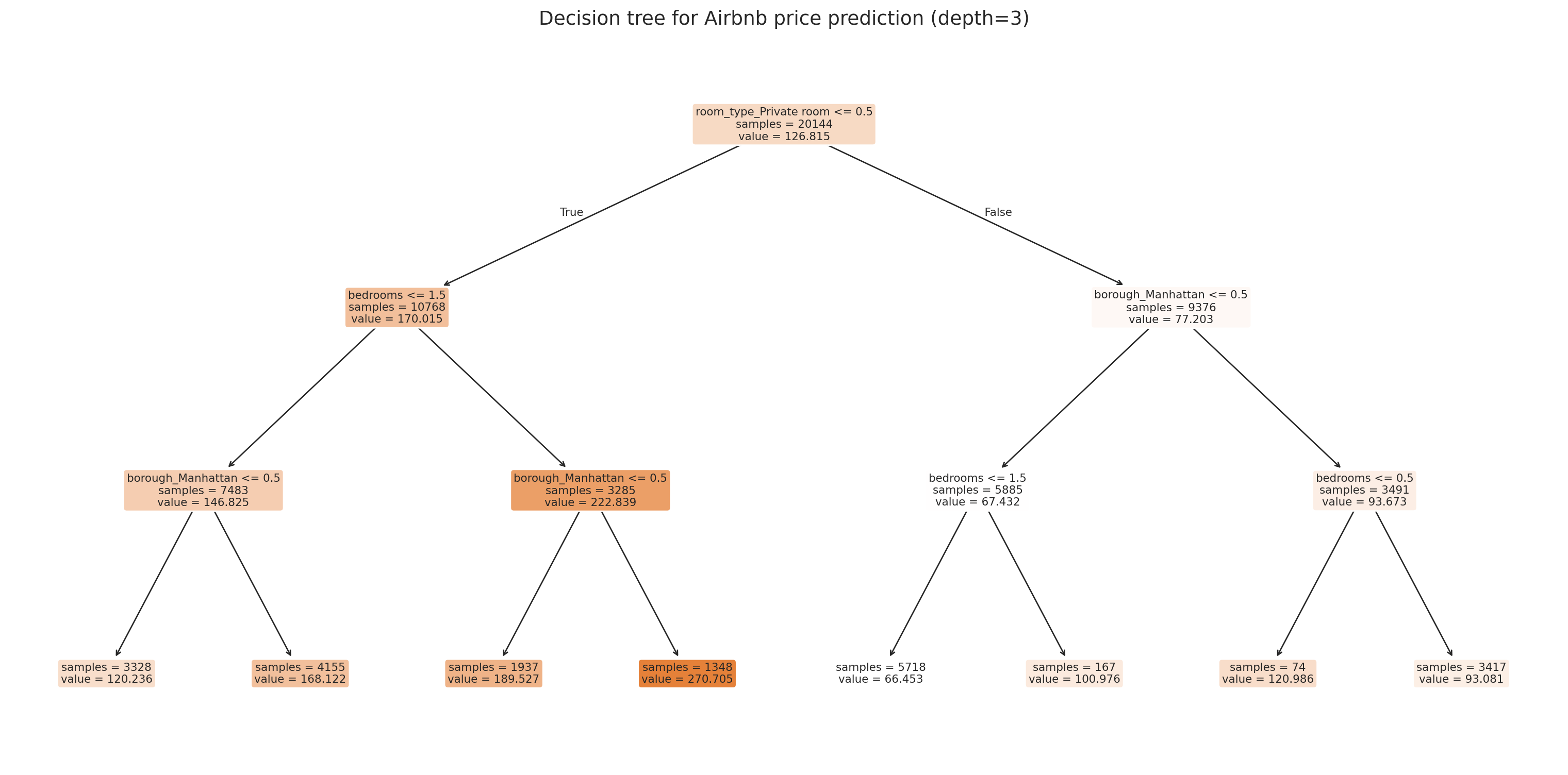
ax.set_title('Decision tree for Airbnb price prediction (depth=3)', fontsize=14)
plt.tight_layout()
plt.show()
```
Each leaf shows the predicted price (the mean of training examples that land there) and how many samples it contains. The tree automatically discovers that room type and borough matter — no one-hot encoding intuition required.
:::{.callout-tip}
## Think About It
The tree picks its own split points. Look at the first split — does it match your intuition about what matters most for price?
:::
### How a decision tree splits
A decision tree partitions the feature space using a **greedy** algorithm. At each node, it considers every feature and every possible threshold, choosing the split that produces the most homogeneous child nodes.
For regression, "homogeneous" means low variance. The algorithm picks the split that minimizes the total squared error in the two child nodes:
$$\min_{j,\, s} \left[ \sum_{x_i \in R_1(j,s)} (y_i - \bar{y}_1)^2 + \sum_{x_i \in R_2(j,s)} (y_i - \bar{y}_2)^2 \right]$$
where $R_1(j,s) = \{x : x_j \le s\}$ and $R_2(j,s) = \{x : x_j > s\}$ are the two regions created by splitting feature $j$ at threshold $s$, and $\bar{y}_1, \bar{y}_2$ are the mean outcomes in each region. Each leaf predicts the mean of the training observations that fall into it.
For classification, the criterion is **Gini impurity** instead of squared error. A node is "pure" if every observation in it has the same label. The Gini index $\hat{p}(1 - \hat{p})$ measures how mixed a node is, where $\hat{p}$ is the fraction of observations with label 1. The algorithm greedily picks splits that maximize the total decrease in impurity.
The process is **recursive**: after the first split creates two child nodes, the algorithm splits each child independently, and so on. The tree grows until a stopping criterion is met — typically a maximum depth or a minimum number of samples per leaf.
```{python}
# Text representation of the tree structure
print(export_text(tree_viz, feature_names=feature_names, max_depth=3))
```
## Overfitting a single tree
A decision tree with no depth limit will keep splitting until every leaf contains a single training observation. The result: perfect training accuracy and terrible generalization. Let's see the damage.
```{python}
# Fit trees at increasing depths and track train vs test R²
depths = [1, 2, 3, 4, 5, 7, 10, 15, 20, None]
depth_labels = [str(d) if d else 'None' for d in depths]
train_r2s = []
test_r2s = []

for d in depths:
    t = DecisionTreeRegressor(max_depth=d, random_state=42)
    t.fit(X_train, y_train)
    train_r2s.append(t.score(X_train, y_train))
    test_r2s.append(t.score(X_test, y_test))
    label = f"depth={str(d):>4s}"
    print(f"{label}:  Train R² = {train_r2s[-1]:.3f}  |  Test R² = {test_r2s[-1]:.3f}")
```
```{python}
fig, ax = plt.subplots(figsize=(10, 5))
x_pos = range(len(depths))
ax.plot(x_pos, train_r2s, 'o-', color='steelblue', linewidth=2, markersize=8, label='Train R²')
ax.plot(x_pos, test_r2s, 's-', color='orangered', linewidth=2, markersize=8, label='Test R²')
ax.set_xticks(x_pos)
ax.set_xticklabels(depth_labels)
ax.set_xlabel('Tree depth (max_depth)')
ax.set_ylabel('R²')
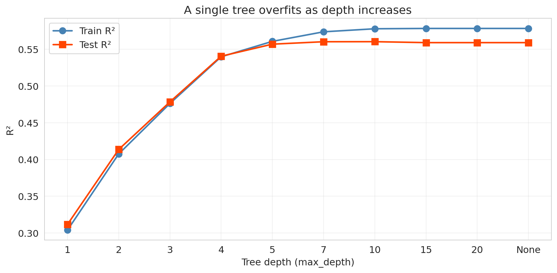
ax.set_title('A single tree overfits as depth increases')
ax.legend(fontsize=12)
ax.grid(True, alpha=0.3)
plt.tight_layout()
plt.show()
```
The pattern is dramatic. Training R² climbs toward 1.0 as the tree memorizes the data. Test R² peaks at a shallow depth and then deteriorates — the tree learns noise rather than signal.
Let's visualize the predictions from a shallow and deep tree to see what overfitting looks like.
```{python}
# Compare shallow vs deep tree predictions along the bedrooms axis
fig, axes = plt.subplots(1, 2, figsize=(14, 5), sharey=True)

# Create prediction grid: vary bedrooms, hold other features at median
median_features = X_train.median()
bedroom_range = np.arange(0, 7, 0.05)
X_slice = pd.DataFrame(
    np.tile(median_features.values, (len(bedroom_range), 1)),
    columns=X_train.columns
)
X_slice['bedrooms'] = bedroom_range

for ax, depth, title in zip(axes,
                             [3, 20],
                             ['Shallow tree (depth=3)', 'Deep tree (depth=20)']):
    t = DecisionTreeRegressor(max_depth=depth, random_state=42)
    t.fit(X_train, y_train)
    preds = t.predict(X_slice)

    ax.scatter(df['bedrooms'] + np.random.normal(0, 0.05, len(df)),
               prices, alpha=0.02, s=3, color='gray', label='data')
    ax.plot(bedroom_range, preds, color='orangered', linewidth=2.5, label=f'depth={depth}')
    ax.set_xlabel('Bedrooms')
    ax.set_ylabel('Predicted price ($)')
    ax.set_title(title)
    ax.legend()
    ax.set_xlim(-0.5, 6.5)

plt.tight_layout()
plt.show()
```
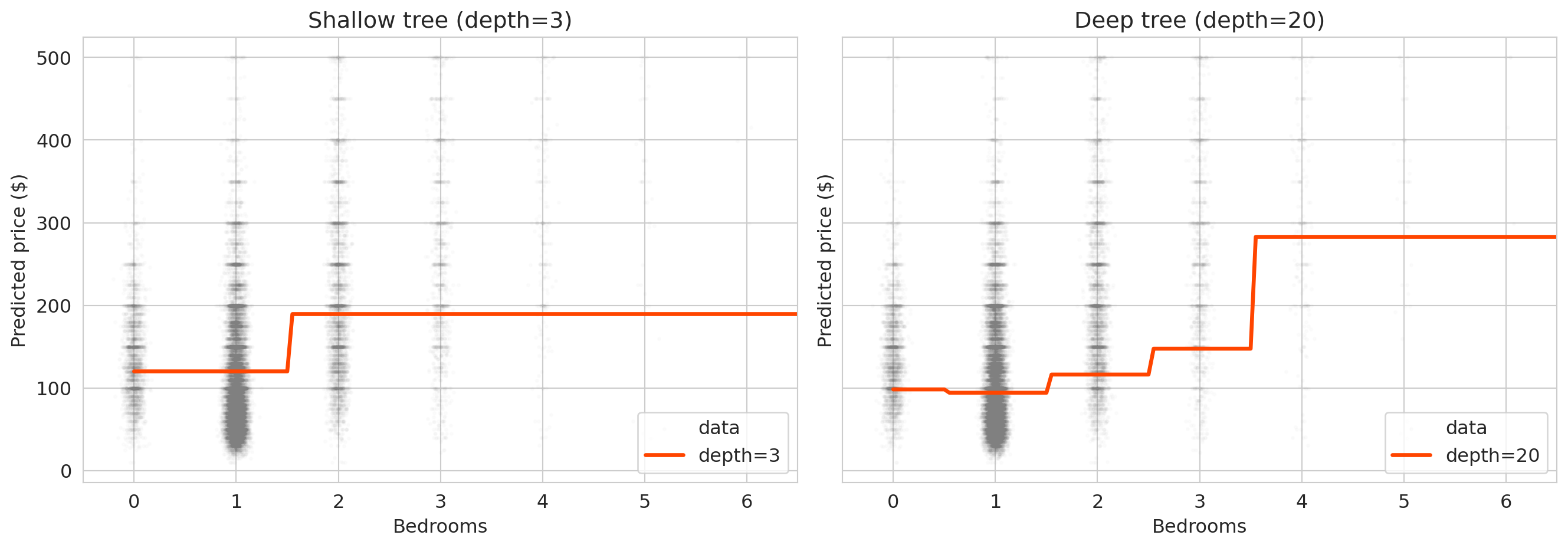
The shallow tree produces smooth, interpretable predictions. The deep tree produces jagged step functions that jump wildly between adjacent bedroom counts — it has memorized the training data's quirks rather than learning the underlying pattern.
:::{.callout-tip}
## Think About It
A deep tree achieves a training R² close to 1.0. Why doesn't that make it a good model? What would you look at to decide when to stop growing the tree?
:::
## Random forests
One tree overfits. What about averaging many trees?
A **random forest** fits hundreds of decision trees, each on a random subset of the data and features, then averages their predictions. The randomness ensures the trees disagree on noise but agree on signal.
```{python}
rf = RandomForestRegressor(n_estimators=100, random_state=42)
rf.fit(X_train, y_train)

rf_train_r2 = rf.score(X_train, y_train)
rf_test_r2 = rf.score(X_test, y_test)

print("Model comparison (test R²):")
print(f"  Decision Tree (depth=4):     {tree_test_r2:.3f}")
print(f"  Random Forest (100 trees):   {rf_test_r2:.3f}")
```
The forest beats the single tree — and we didn't tune any hyperparameters beyond the number of trees.
### How random forests work: bagging + feature subsampling
A random forest combines two ideas:
1. **Bagging** (bootstrap aggregating): each tree trains on a different bootstrap sample — a random draw (with replacement) from the training data. Each sample is the same size as the original dataset but contains some observations multiple times and omits others.
2. **Feature subsampling**: at each split, the tree considers only a random subset of features (typically $\sqrt{p}$ out of $p$ total features). This forces the trees to find different splits, reducing the correlation between trees.
The ensemble prediction is the average of all individual tree predictions (for regression) or majority vote (for classification).
Each individual tree is overfit — it has memorized the noise in its particular bootstrap sample. Averaging works because different trees memorize *different* noise.
### More trees never hurts
Let's train random forests with increasing numbers of trees and track test performance.
```{python}
# Build feature matrix for the full train/test sets
n_trees_list = [1, 5, 10, 25, 50, 100, 200, 500]
rf_test_scores = []

for n_trees in n_trees_list:
    rf_temp = RandomForestRegressor(n_estimators=n_trees, random_state=42, n_jobs=-1)
    rf_temp.fit(X_train, y_train)
    score = rf_temp.score(X_test, y_test)
    rf_test_scores.append(score)
    print(f"n_estimators = {n_trees:>3d}: Test R² = {score:.4f}")
```
```{python}
fig, ax = plt.subplots(figsize=(10, 5))

ax.plot(n_trees_list, rf_test_scores, 'o-', color='forestgreen', linewidth=2.5, markersize=10)
ax.set_xlabel('Number of trees (n_estimators)')
ax.set_ylabel('Test R²')
ax.set_title('Random forest: more trees = better or flat — never worse')
ax.set_xscale('log')
ax.set_xticks(n_trees_list)
ax.set_xticklabels(n_trees_list)
ax.grid(True, alpha=0.3)
plt.tight_layout()
plt.show()
```
No U-shape! The test R² increases and then plateaus. Adding more trees never hurts — it just stops helping. The pattern is fundamentally different from the polynomial story in [Chapter 5](lec05-feature-engineering.qmd), where higher polynomial degrees eventually *destroyed* test performance. (Caveat: this "more is never worse" property is specific to bagging/random forests. For *gradient boosting*, which we'll meet in [Chapter 17](lec17-automl-llms.qmd), adding too many trees *can* overfit.)
### Individual trees are overfit; their average is smooth
To understand why averaging works, let's look at what individual trees actually predict. We'll train 5 decision trees on bootstrap samples and plot their predictions along a 1D slice: price vs. bedrooms, holding other features at their median values.
```{python}
# Create a 1D prediction slice: vary bedrooms, hold everything else at median
median_features = X_train.median()
bedroom_range = np.arange(0, 7, 0.1)
X_slice = pd.DataFrame(
np.tile(median_features.values, (len(bedroom_range), 1)),
columns=X_train.columns
)
X_slice['bedrooms'] = bedroom_range
# Train 5 individual trees on bootstrap samples
np.random.seed(42)
fig, ax = plt.subplots(figsize=(10, 6))
individual_preds = []
for i in range(5):
# Bootstrap sample
boot_idx = np.random.choice(len(X_train), size=len(X_train), replace=True)
X_boot = X_train.iloc[boot_idx]
y_boot = y_train.iloc[boot_idx]
tree_i = DecisionTreeRegressor(max_depth=None, random_state=i)
tree_i.fit(X_boot, y_boot)
preds = tree_i.predict(X_slice)
individual_preds.append(preds)
ax.plot(bedroom_range, preds, alpha=0.4, linewidth=1.2, label=f'Tree {i+1}')
# Average prediction
avg_preds = np.mean(individual_preds, axis=0)
ax.plot(bedroom_range, avg_preds, color='black', linewidth=3, label='Average (5 trees)', zorder=5)
ax.set_xlabel('Bedrooms')
ax.set_ylabel('Predicted price ($)')
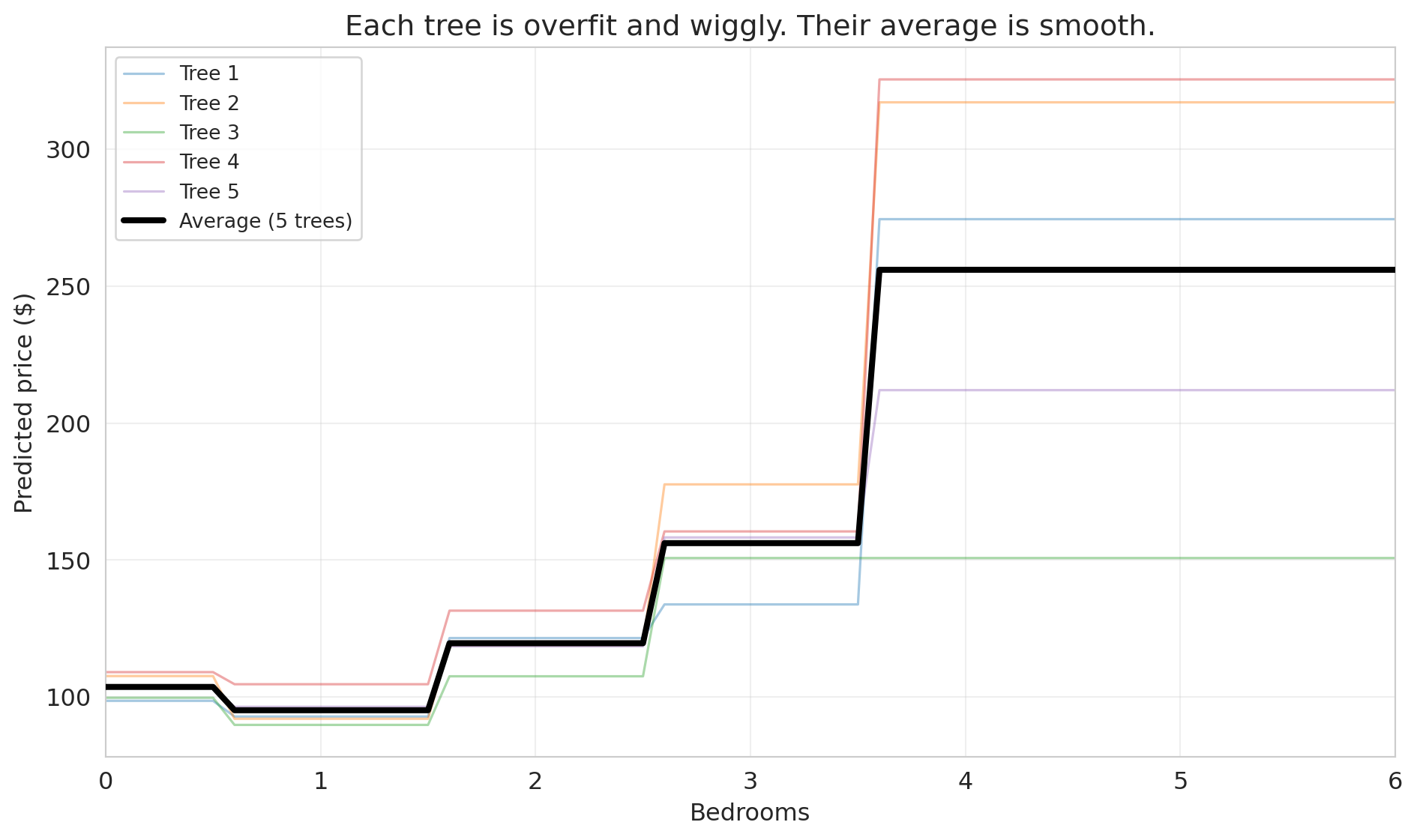
ax.set_title('Each tree is overfit and wiggly. Their average is smooth.')
ax.legend(fontsize=10, loc='upper left')
ax.set_xlim(0, 6)
ax.grid(True, alpha=0.3)
plt.tight_layout()
plt.show()
```
Each individual tree (thin colored lines) is wiggly and overfit — it has memorized the quirks of its particular bootstrap sample. But their *errors point in different directions*. One tree might predict too high for 3-bedroom listings while another predicts too low. When we average them, the noise cancels out, and what remains is the genuine signal.
The core insight of **bagging** (bootstrap aggregating): averaging many overfit models reduces variance without increasing bias. It's the same principle behind asking 100 people to estimate the weight of a cow at a county fair — individual guesses vary wildly, but the average is remarkably accurate.
## Random forest as benchmark
How does the random forest compare to the hand-engineered linear model from [Chapter 5](lec05-feature-engineering.qmd)? Let's put them head to head.
```{python}
# Linear model with interactions (same as Chapter 5)
borough_dummies = pd.get_dummies(df['borough'], drop_first=True)
interactions = borough_dummies.multiply(df['bedrooms'], axis=0)
interactions.columns = [f'bedrooms_x_{col}' for col in interactions.columns]
X_interact = pd.concat([X_base, interactions], axis=1)

lm_interact = LinearRegression().fit(
    X_interact.loc[X_train.index], y_train
)
lm_test_r2 = r2_score(y_test, lm_interact.predict(X_interact.loc[X_test.index]))

# Random forest (already fit above)
print("Test R² comparison:")
print(f"  Linear model (bedrooms + bath + room + borough):         {r2_score(y_test, LinearRegression().fit(X_train, y_train).predict(X_test)):.3f}")
print(f"  Linear model + interactions:                             {lm_test_r2:.3f}")
print(f"  Decision tree (depth=4):                                 {tree_test_r2:.3f}")
print(f"  Random forest (100 trees):                               {rf_test_r2:.3f}")
```
The random forest wins — and required zero feature engineering. No polynomial terms, no interaction terms, no decisions about which features to cross. For tabular prediction tasks, a random forest is a strong default benchmark: if your hand-crafted model can't beat it, the engineering effort may not be worthwhile.
:::{.callout-tip}
## Think About It
The random forest beats the linear model with interactions. Does that mean linear models are useless? What advantages might a linear model still have? (Hint: think about interpretability and coefficient meaning.)
:::
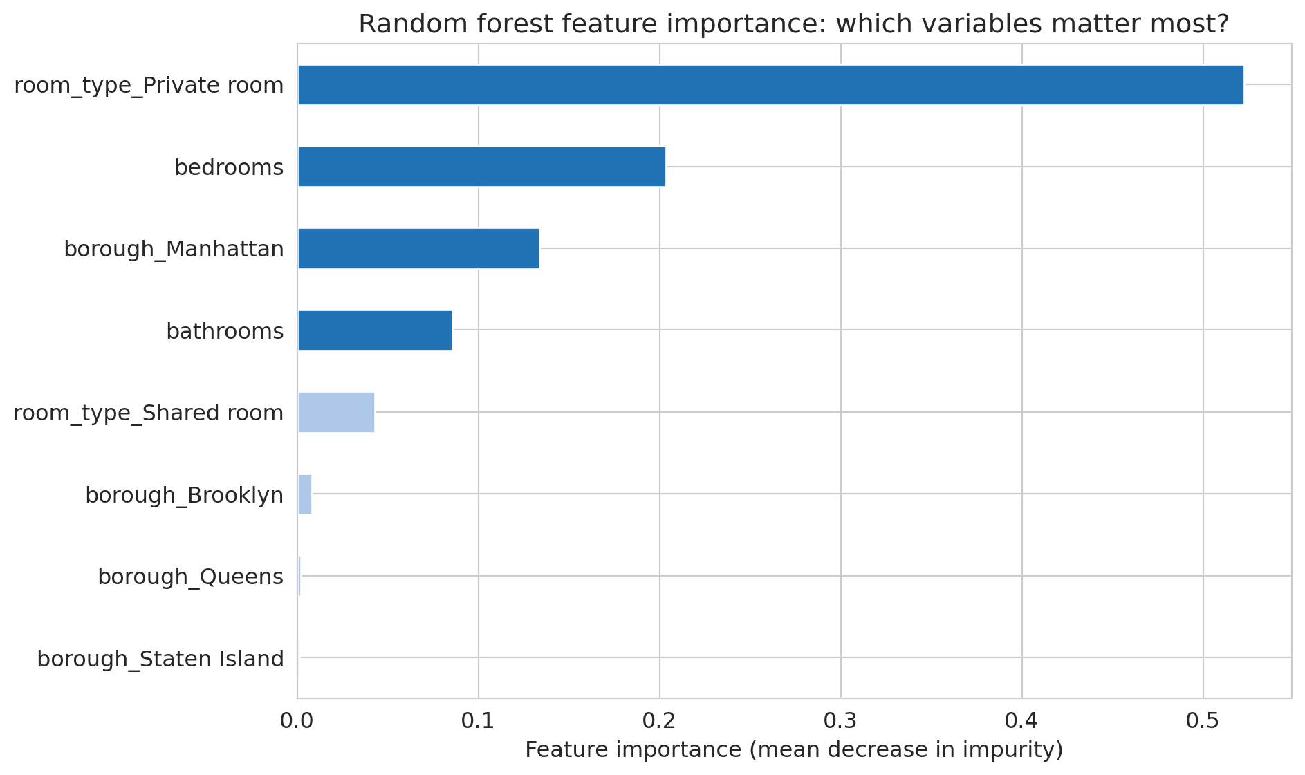
## Feature importance
A random forest is harder to interpret than a linear regression — you can't point to a single coefficient and say "each bedroom adds \$X." But the forest does tell you which features it relies on most.
**Feature importance** measures how much each feature contributes to reducing prediction error across all trees in the forest. Specifically, scikit-learn's `feature_importances_` reports the **mean decrease in impurity (MDI)**: for each feature, it averages the total reduction in squared error (or Gini impurity) across every split in every tree that uses that feature.
```{python}
# Feature importance from the random forest
importances = pd.Series(rf.feature_importances_, index=feature_names)
importances_sorted = importances.sort_values()

fig, ax = plt.subplots(figsize=(10, 6))
colors = ['#2171b5' if v > importances.median() else '#aec7e8' for v in importances_sorted]
importances_sorted.plot(kind='barh', ax=ax, color=colors, edgecolor='white')
ax.set_xlabel('Feature importance (mean decrease in impurity)')
ax.set_title('Random forest feature importance: which variables matter most?')
plt.tight_layout()
plt.show()
```
Compare this to a linear regression's coefficients. In a linear model, the coefficient on `bedrooms` tells you the marginal effect of one additional bedroom, holding all else equal — a causal-flavored interpretation (though only valid under strong assumptions). Feature importance tells you something different: how much the forest *uses* a feature for splitting, which reflects both direct effects and interactions. A feature can be important without having a simple linear relationship with the outcome.
:::{.callout-warning}
## MDI can be misleading
Mean decrease in impurity is biased toward features with many possible split points (high-cardinality features). A feature with 100 unique values gets more chances to be selected than a binary feature, even if both are equally predictive. **Permutation importance** — measuring how much test accuracy drops when a feature is randomly shuffled — is a more reliable alternative for comparing features on different scales.
:::
### How trees handle missing data
Unlike linear regression, which requires complete data for every row, decision trees can handle missing values directly. Different implementations use different strategies:
**Surrogate splits.** When a tree encounters a missing value at a split node, it looks for an alternative feature that produces a similar partition. If the best split is on `bedrooms` and a row has a missing bedroom count, the tree might split on `accommodates` instead (a correlated feature). The original CART algorithm uses this approach. (Note: scikit-learn's `DecisionTreeClassifier` does *not* implement surrogate splits — it requires complete data. Use `HistGradientBoostingClassifier` for native missing-value support.)
**Native missing-value handling.** XGBoost and LightGBM go further: during training, they learn which branch (left or right) missing values should follow at each split, choosing whichever direction reduces the loss more. No imputation needed — the algorithm treats "missing" as just another value to route.
**Why trees handle this well.** A decision tree asks a yes/no question at each node. Missing values simply need a rule for which branch to follow. Linear models, by contrast, need a numeric value to multiply by a coefficient — a missing value breaks the computation entirely.
:::{.callout-tip}
## Think About It
If 30% of your `bedrooms` column is missing and you impute with the median before fitting a tree, what information have you destroyed? Would the tree have been better off seeing the missingness directly?
:::
In practice, tree-based models (especially gradient-boosted trees like XGBoost) are the most popular choice for tabular data with missing values — precisely because they don't require the analyst to make imputation decisions that could introduce bias.
::::{.callout-note}
## Preview: classification
Everything above predicts a continuous number (price). **Classification** predicts a discrete category instead — "expensive or not," "spam or not." The same tree-based machinery applies: a classification tree predicts the majority class in each leaf, and a random forest classifier uses majority vote across trees. We develop classification properly with logistic regression in [Chapter 13](lec13-classification.qmd); for projects before then, `RandomForestClassifier` from scikit-learn works out of the box with the same `fit`/`score` interface.
::::
## Key takeaways
- **Decision trees find splits automatically — no manual feature engineering.** The model examines every feature and every threshold, choosing splits that minimize prediction error. No need for one-hot encoding, polynomial terms, or interaction terms.
- **A single deep tree overfits: perfect training score, poor test score.** With no depth limit, a tree memorizes the training data. The training R² approaches 1 while the test R² deteriorates.
- **Random forests average many overfit trees; the average is stable.** Each tree sees different bootstrap data and different feature subsets. The noise cancels; the signal persists.
- **More trees never hurts (unlike more polynomial features).** Test R² improves and then plateaus as we add trees — no U-shaped overfitting curve.
- **Trees handle missing data and categories natively.** Surrogate splits and native missing-value routing make imputation unnecessary. Categories can be split directly without one-hot encoding.
- **Feature importance ranks which variables the forest relies on.** Mean decrease in impurity (MDI) measures how much each feature contributes to reducing prediction error, but beware of bias toward high-cardinality features.
## Study guide
### Key ideas
- **Decision tree** — a model that recursively partitions the feature space by asking if/then questions about individual features, predicting the mean outcome (regression) or majority class (classification) in each leaf.
- **Recursive splitting** — the greedy algorithm that builds a tree: at each node, choose the feature and threshold that minimize prediction error in the child nodes.
- **Overfitting in trees** — a tree with no depth limit memorizes the training data (training R² ≈ 1) but performs poorly on new data. Controlling depth limits this memorization.
- **Bagging (bootstrap aggregating)** — training many models on different bootstrap samples of the data and averaging their predictions. Reduces variance without increasing bias.
- **Feature subsampling** — at each split, considering only a random subset of features. This decorrelates the trees in the ensemble, making the average more effective.
- **Random forest** — an ensemble of bagged decision trees with feature subsampling. More trees = better or flat, never worse.
- **Feature importance (MDI)** — mean decrease in impurity: the average reduction in squared error (or Gini impurity) across all splits using a given feature. Biased toward high-cardinality features; permutation importance is a more robust alternative.
- **Missing data in trees** — trees handle missing values natively via surrogate splits or learned missing-value routing, unlike linear models that require imputation.
### Computational tools
- `DecisionTreeRegressor(max_depth=4).fit(X, y)` — fits a regression tree with controlled depth
- `RandomForestRegressor(n_estimators=100).fit(X, y)` — fits a random forest; more trees = better or flat, never worse
- `plot_tree(tree, feature_names=..., filled=True)` — visualizes a fitted decision tree
- `export_text(tree, feature_names=...)` — prints the tree's decision rules as text
- `rf.feature_importances_` — array of feature importance scores (mean decrease in impurity)
- `train_test_split(X, y, test_size=0.3)` — splits data into training and test sets for honest evaluation
### For the quiz
You are responsible for: how a decision tree splits (greedy recursive partitioning), why deep trees overfit, how bagging and feature subsampling combine to form a random forest, why adding more trees never hurts, feature importance interpretation, and the advantages of trees over linear models for handling missing data and categorical features.