---
title: "Trees, Validation, and Bias-Variance"
execute:
enabled: true
jupyter: python3
---
A hospital is considering an AI system that predicts which patients will develop sepsis — a life-threatening condition where early intervention is critical. The vendor, Epic Systems, reports an AUC of 0.76–0.83. The hospital buys the system and deploys it. What questions should they have asked?
When researchers at Michigan Medicine independently evaluated the model on 27,697 hospitalized patients, they found an AUC of just 0.63 — barely better than chance. The model missed 67% of sepsis cases while firing false alerts on 18% of all hospitalizations, drowning nurses in alarms for patients who were fine.^[Wong et al., "External Validation of a Widely Implemented Proprietary Sepsis Prediction Model in Hospitalized Patients," *JAMA Internal Medicine*, 2021. <https://pmc.ncbi.nlm.nih.gov/articles/PMC8218233/>] The root cause: Epic evaluated the model on data similar to its training data, not on an independent external test set. The model had learned patterns specific to one hospital system's patient population and coding practices. Those patterns didn't generalize.
The Epic sepsis model is not an isolated failure. Dermatology AI systems have reported 90%+ accuracy on light skin tones but as low as 17% on dark skin, because the test sets didn't reflect the diversity of the deployment population.^[Daneshjou et al., "Disparities in Dermatology AI Performance on a Diverse, Curated Clinical Image Set," *Science Advances*, 2022.] Amazon built an AI recruiting tool that achieved high accuracy but systematically penalized resumes containing the word "women's" — the model had learned to replicate historical hiring bias embedded in its training data, and the company scrapped it.^[Dastin, "Amazon scraps secret AI recruiting tool that showed bias against women," *Reuters*, 2018.] In each case, the model looked good on data it had already seen but failed on the data that mattered.
In [Chapter 6](lec06-feature-engineering.qmd), we engineered features — dummies, polynomials, interactions — and saw that a linear model can capture surprisingly complex patterns. We also met decision trees and random forests, which engineer features automatically. But we've been measuring performance on the *same data we trained on*. Evaluating a model on its training data is like grading a student on the questions they've already seen — of course they'll do well. The question the hospital *should* have asked is the question this chapter answers: **does this model generalize?** We'll develop the tools to answer it: train/test splits, cross-validation, and the bias-variance tradeoff that explains why more complex models don't always win.
:::{.callout-note}
## All Models Are Wrong
"All models are wrong, but some are useful." — George Box (1976)
Every model simplifies reality. The question is never *whether* a model is exactly right — no model is. The question is whether the model's approximation is close enough to be useful for the decision at hand. The entire machinery of validation exists to answer that question.
:::
```{python}
import numpy as np
import pandas as pd
import matplotlib.pyplot as plt
import seaborn as sns
from sklearn.linear_model import LinearRegression, Lasso, LassoCV
from sklearn.ensemble import RandomForestRegressor
from sklearn.tree import DecisionTreeRegressor
from sklearn.preprocessing import PolynomialFeatures
from sklearn.model_selection import cross_val_score, train_test_split
from sklearn.metrics import r2_score, mean_squared_error
import warnings
warnings.filterwarnings('ignore')
sns.set_style('whitegrid')
plt.rcParams['figure.figsize'] = (7, 4.5)
plt.rcParams['font.size'] = 12

DATA_DIR = 'data'
```
## Adding features: diminishing returns
Adding features always improves training $R^2$. But does it improve predictions on *new* data — and if so, by how much?
Let's find out. We'll build feature matrices at six different complexity levels — from minimal (just bedrooms and bathrooms) to kitchen-sink (all pairwise interactions) — and track performance on both the training and test sets.
```{python}
# Load Airbnb data (same setup as Chapter 6)
listings = pd.read_csv(f'{DATA_DIR}/airbnb/listings.csv', low_memory=False)

cols = ['price', 'bedrooms', 'bathrooms', 'room_type', 'neighbourhood_group_cleansed']
df = listings[cols].dropna().copy()
df = df.rename(columns={'neighbourhood_group_cleansed': 'borough'})

# Clean price column
df['price'] = df['price'].astype(str).str.replace('[$,]', '', regex=True).astype(float)

# Filter to reasonable prices
df = df[df['price'].between(10, 500)].reset_index(drop=True)
y = df['price']

print(f"{len(df):,} listings")
df.head()
```
Here's the plan: six levels of model complexity, each one adding to the previous.
| Level | What it adds | Intuition |
|-------|-------------|-----------|
| 1 | bedrooms + bathrooms | Raw numeric features only |
| 2 | + room type dummies | Different baseline by listing type |
| 3 | + borough dummies | Different baseline by location |
| 4 | + bedroom x borough interactions | Different slopes by location |
| 5 | + polynomial features (degree 3) | Nonlinear numeric effects |
| 6 | all pairwise interactions | Everything interacts with everything |
```{python}
def build_features(data, level):
    """Build feature matrices at different complexity levels."""
    num = data[['bedrooms', 'bathrooms']].copy()

    if level == 1:
        return num

    room = pd.get_dummies(data['room_type'], drop_first=True, prefix='room')
    if level == 2:
        return pd.concat([num, room], axis=1)

    borough = pd.get_dummies(data['borough'], drop_first=True, prefix='boro')
    if level == 3:
        return pd.concat([num, room, borough], axis=1)

    # Level 4: add bedroom x borough interactions
    inter = borough.multiply(data['bedrooms'], axis=0)
    inter.columns = [f'{c}_x_bed' for c in inter.columns]
    if level == 4:
        return pd.concat([num, room, borough, inter], axis=1)

    # Level 5: add polynomial features (degree 3) on numeric columns
    poly = PolynomialFeatures(degree=3, include_bias=False)
    num_poly = pd.DataFrame(
        poly.fit_transform(num),
        columns=[f'poly_{i}' for i in range(poly.n_output_features_)],
        index=data.index
    )
    if level == 5:
        return pd.concat([num_poly, room, borough, inter], axis=1)

    # Level 6: kitchen-sink — all pairwise interactions
    base = pd.concat([num, room, borough], axis=1)
    poly_all = PolynomialFeatures(degree=2, interaction_only=True, include_bias=False)
    all_inter = pd.DataFrame(poly_all.fit_transform(base), index=data.index)
    return all_inter
```
Now the critical step: **split the data before fitting any models.** We train on 70% and evaluate on the held-out 30%. The test set simulates "new data" we haven't seen.
```{python}
# Split into train and test FIRST — before looking at any results
np.random.seed(42)
train_idx, test_idx = train_test_split(range(len(df)), test_size=0.3, random_state=42)

df_train = df.iloc[train_idx].reset_index(drop=True)
df_test = df.iloc[test_idx].reset_index(drop=True)
y_train = df_train['price']
y_test = df_test['price']

print(f"Train: {len(df_train):,}  |  Test: {len(df_test):,}")
```
We fit a `LinearRegression` at each complexity level and record both training and test $R^2$.
```{python}
model_names = [
    '1: bedrooms+bath',
    '2: + room_type',
    '3: + borough',
    '4: + interactions',
    '5: + polynomials',
    '6: all pairwise'
]

train_r2s = []
test_r2s = []
n_features_list = []

for level in range(1, 7):
    X_tr = build_features(df_train, level)
    X_te = build_features(df_test, level)

    m = LinearRegression().fit(X_tr, y_train)

    train_r2s.append(m.score(X_tr, y_train))
    test_r2s.append(r2_score(y_test, m.predict(X_te)))
    n_features_list.append(X_tr.shape[1])

results_df = pd.DataFrame({
    'Model': model_names,
    'Features': n_features_list,
    'Train R²': [f'{r:.4f}' for r in train_r2s],
    'Test R²': [f'{r:.4f}' for r in test_r2s]
})
print(results_df.to_string(index=False))
```
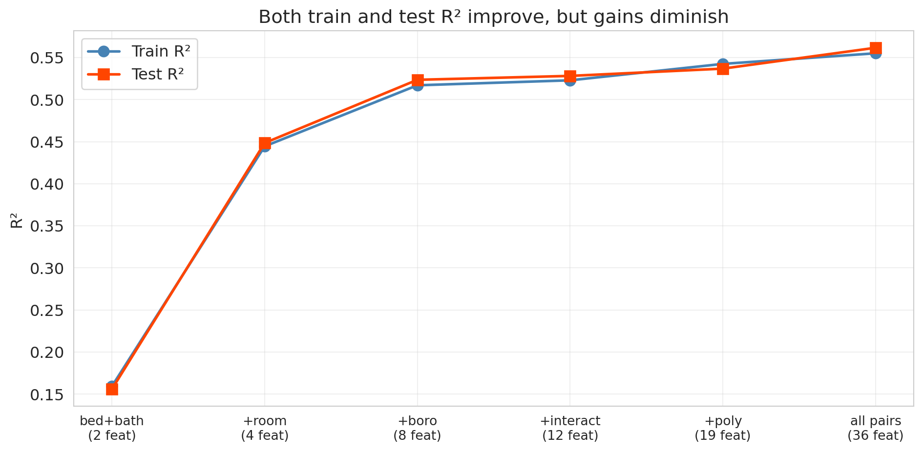
Training $R^2$ increases monotonically, as guaranteed. What about test $R^2$?
```{python}
fig, ax = plt.subplots(figsize=(10, 5))

x_pos = range(len(model_names))
ax.plot(x_pos, train_r2s, 'o-', color='steelblue', linewidth=2, markersize=8, label='Train R²')
ax.plot(x_pos, test_r2s, 's-', color='orangered', linewidth=2, markersize=8, label='Test R²')

ax.set_xticks(x_pos)
ax.set_xticklabels([f'{n}\n({nf} feat)' for n, nf in zip(
    ['bed+bath', '+room', '+boro', '+interact', '+poly', 'all pairs'],
    n_features_list)], fontsize=10)
ax.set_ylabel('R²')
ax.set_title('Both train and test R² improve, but gains diminish')
ax.legend(fontsize=12)
ax.grid(True, alpha=0.3)
plt.tight_layout()
plt.show()
```
Look at the gap between the blue line (train) and the red line (test). Both keep climbing — each new batch of features captures real signal. But notice the **diminishing returns**: the jump from Level 1 to Level 3 is enormous, while Levels 4 through 6 add only marginal improvement. The train-test gap also widens slightly as we add more features, hinting that the model is beginning to fit noise alongside signal. With enough data (we have over 20,000 listings here), that noise-fitting doesn't dominate — all six feature sets genuinely help. But what happens with a smaller dataset or far more features? That's where overfitting becomes dramatic.
:::{.callout-tip}
## Think About It
Why does the training $R^2$ always go up? Adding a feature can only help the model fit the training data better — in the worst case, the model sets that feature's coefficient to zero.
:::
### When more features = worse predictions
The six-level experiment didn't overfit because we had plenty of data relative to the number of features (36 features for over 20,000 listings). Let's see what happens when that ratio flips. We'll use a smaller sample (500 listings) and increase the polynomial degree from 1 to 7, creating thousands of features from only 300 training observations. With far more features than data points, the overfitting is dramatic.
```{python}
np.random.seed(42)

# Smaller sample — overfitting is more dramatic with less data
df_small = df.sample(500, random_state=42).reset_index(drop=True)
y_small = df_small['price']
train_i, test_i = train_test_split(range(len(df_small)), test_size=0.4, random_state=42)

# Base features: numeric + dummies
base_cat = pd.get_dummies(df_small[['room_type', 'borough']], drop_first=True)
X_base_small = pd.concat([df_small[['bedrooms', 'bathrooms']], base_cat], axis=1)

degrees = [1, 2, 3, 4, 5, 6, 7]
train_scores_poly = []
test_scores_poly = []
n_feat_poly = []

for deg in degrees:
    poly = PolynomialFeatures(degree=deg, include_bias=False)
    X_poly = pd.DataFrame(poly.fit_transform(X_base_small))
    n_feat_poly.append(X_poly.shape[1])

    X_tr = X_poly.iloc[train_i]
    X_te = X_poly.iloc[test_i]
    y_tr = y_small.iloc[train_i]
    y_te = y_small.iloc[test_i]

    m = LinearRegression().fit(X_tr, y_tr)
    train_scores_poly.append(m.score(X_tr, y_tr))
    test_r2 = r2_score(y_te, m.predict(X_te))
    test_scores_poly.append(test_r2)

    print(f"Degree {deg}: {X_poly.shape[1]:5d} features | "
          f"Train R² = {train_scores_poly[-1]:.3f} | Test R² = {test_r2:.3f}")
```
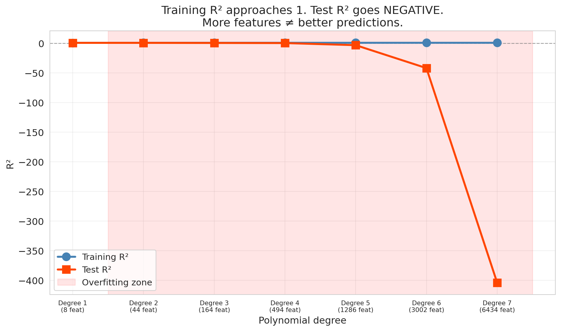
By degree 7, the model has over 6,000 features for only 300 training observations. The result is catastrophic overfitting.
```{python}
fig, ax = plt.subplots(figsize=(10, 6))

ax.plot(degrees, train_scores_poly, 'o-', color='steelblue', linewidth=2.5, markersize=10,
        label='Training R²', zorder=3)
ax.plot(degrees, test_scores_poly, 's-', color='orangered', linewidth=2.5, markersize=10,
        label='Test R²', zorder=3)

# Shade the overfitting region
best_test_idx = np.argmax(test_scores_poly)
if best_test_idx < len(degrees) - 1:
    ax.axvspan(degrees[best_test_idx] + 0.5, degrees[-1] + 0.5, alpha=0.1, color='red',
               label='Overfitting zone')

ax.axhline(y=0, color='gray', linestyle='--', linewidth=1, alpha=0.7)
ax.set_xlabel('Polynomial degree')
ax.set_ylabel('R²')
ax.set_title('Training R² approaches 1. Test R² goes NEGATIVE.\nMore features ≠ better predictions.')
ax.legend(fontsize=11)
ax.set_xticks(degrees)
ax.set_xticklabels([f'Degree {d}\n({n} feat)' for d, n in zip(degrees, n_feat_poly)],
                   fontsize=8)
ax.grid(True, alpha=0.3)
plt.tight_layout()
plt.show()
```
The training $R^2$ approaches 1 — the model nearly perfectly memorizes the training data. Meanwhile, the test $R^2$ plummets, eventually going *negative*.
Wait — can $R^2$ be negative? Yes, on test data. On training data, $R^2$ is always between 0 and 1 (when the model includes an intercept). On test data, no such guarantee holds. Recall that $R^2 = 1 - \text{SS}_{\text{res}} / \text{SS}_{\text{tot}}$. When a model's predictions on new data are worse than simply predicting the mean every time, the residual sum of squares exceeds the total sum of squares, and $R^2$ drops below zero. Negative $R^2$ on test data means the model is worse than predicting the mean — a sign of catastrophic overfitting.
## The bias-variance tradeoff
The polynomial experiment showed a striking pattern: test error first decreased and then increased as models got more complex. Why? The answer is one of the most important ideas in all of applied statistics: the **bias-variance tradeoff**.
:::{.callout-important}
## Definition: Bias and Variance
Two sources of prediction error:
- **Bias** is the error from oversimplifying. The model can't capture the true pattern. High bias corresponds to **underfitting** — like fitting a straight line through a curved relationship.
- **Variance** is the error from over-complicating. The model is so flexible that it's too sensitive to the particular training data it happened to see. High variance corresponds to **overfitting** — the model learns noise as if it were signal.
:::
| | Too few features | Just right | Too many features |
|---|---|---|---|
| **Bias** | High (underfitting) | Low | Low |
| **Variance** | Low | Low | High (overfitting) |
| **Test error** | High | **Low** | High |
For mean squared error, the decomposition is exact:
$$\text{Expected test error} = \text{Bias}^2 + \text{Variance} + \sigma^2$$
The first two terms depend on the model. The third term, $\sigma^2$, is the **irreducible noise** — inherent randomness in the outcome that no model can eliminate. Even a perfect model that recovers the true relationship still faces $\sigma^2$. Simple models have high bias but low variance. Complex models have low bias but high variance. The best model minimizes the sum of the first two terms; $\sigma^2$ sets the floor. A more advanced course will formalize this decomposition mathematically and use it to analyze regularization methods like lasso and ridge.
:::{.callout-tip}
## Think About It
In the polynomial experiment above, which degrees had high bias? Which had high variance? Where was the sweet spot?
:::
:::{.callout-note}
## Preview: regularization as bias-variance control
Another approach to controlling overfitting adds a **penalty** directly to the loss function. **Ridge regression** (L2 penalty) shrinks coefficients toward zero; **lasso** (L1 penalty) can shrink them exactly to zero, performing feature selection automatically. The bias-variance tradeoff governs the penalty strength: too little penalty and the model overfits (high variance); too much and it underfits (high bias). We introduce lasso later in this lecture and develop regularization more fully in a later course.
:::
## Train, validation, and test sets
Before introducing cross-validation, we need to distinguish three roles that held-out data can play.
:::{.callout-important}
## Definition: The Three-Way Split
- **Training set** — the data the model learns from.
- **Validation set** — held-out data used to *choose* model complexity (number of features, regularization strength, tree depth). The modeler sees validation scores and adjusts accordingly.
- **Test set** — held-out data touched *only once*, at the very end, to report final performance. No modeling decisions depend on the test set.
:::
Why not just two sets? If we use the test set to choose among models, we are implicitly fitting to the test set. The reported "test" performance becomes optimistic — it no longer estimates how the model will perform on truly unseen data. A dedicated validation set absorbs the cost of model selection so the test set remains pristine.
In practice, a common split is 60% train / 20% validation / 20% test. Our earlier 70/30 split conflated validation and test — acceptable for a first look, but not for rigorous deployment. Cross-validation, introduced next, offers a more data-efficient alternative to a fixed validation set.
## Cross-validation
A single train/test split is noisy — we might get lucky or unlucky. Maybe our test set happened to contain easy-to-predict listings, or maybe the opposite. How do we get a more stable estimate of out-of-sample performance?
**Cross-validation** (CV) solves this problem by systematically rotating which data serves as the test set.
### How 5-fold CV works
1. Split the data randomly into 5 equal-sized **folds**
2. For each fold $k = 1, \ldots, 5$:
- Train the model on the other 4 folds
- Test on fold $k$ and record the score
3. Report the average of the 5 test scores
```
Fold 1:  [TEST ]  [train]  [train]  [train]  [train]   → score_1
Fold 2:  [train]  [TEST ]  [train]  [train]  [train]   → score_2
Fold 3:  [train]  [train]  [TEST ]  [train]  [train]   → score_3
Fold 4:  [train]  [train]  [train]  [TEST ]  [train]   → score_4
Fold 5:  [train]  [train]  [train]  [train]  [TEST ]   → score_5
                                                  Average → CV score
```
Every observation is in the test set exactly once. The average of 5 scores is much more stable than any single train/test split. (The extreme case is **leave-one-out CV** (LOO-CV), where $k = n$ — every observation gets its own fold. LOO-CV has low bias but high variance across folds, and is computationally expensive for large datasets. Five or ten folds is the usual practical choice.)
Let's apply 5-fold CV to our six complexity levels:
```{python}
cv_results = []
for level in range(1, 7):
    X_all = build_features(df, level)
    scores = cross_val_score(LinearRegression(), X_all, y, cv=5, scoring='r2')
    cv_results.append({
        'model': model_names[level-1],
        'features': X_all.shape[1],
        'cv_mean': scores.mean(),
        'cv_std': scores.std()
    })
    print(f"Level {level}: CV R² = {scores.mean():.4f} ± {scores.std():.4f}  ({X_all.shape[1]} features)")

cv_df = pd.DataFrame(cv_results)
```
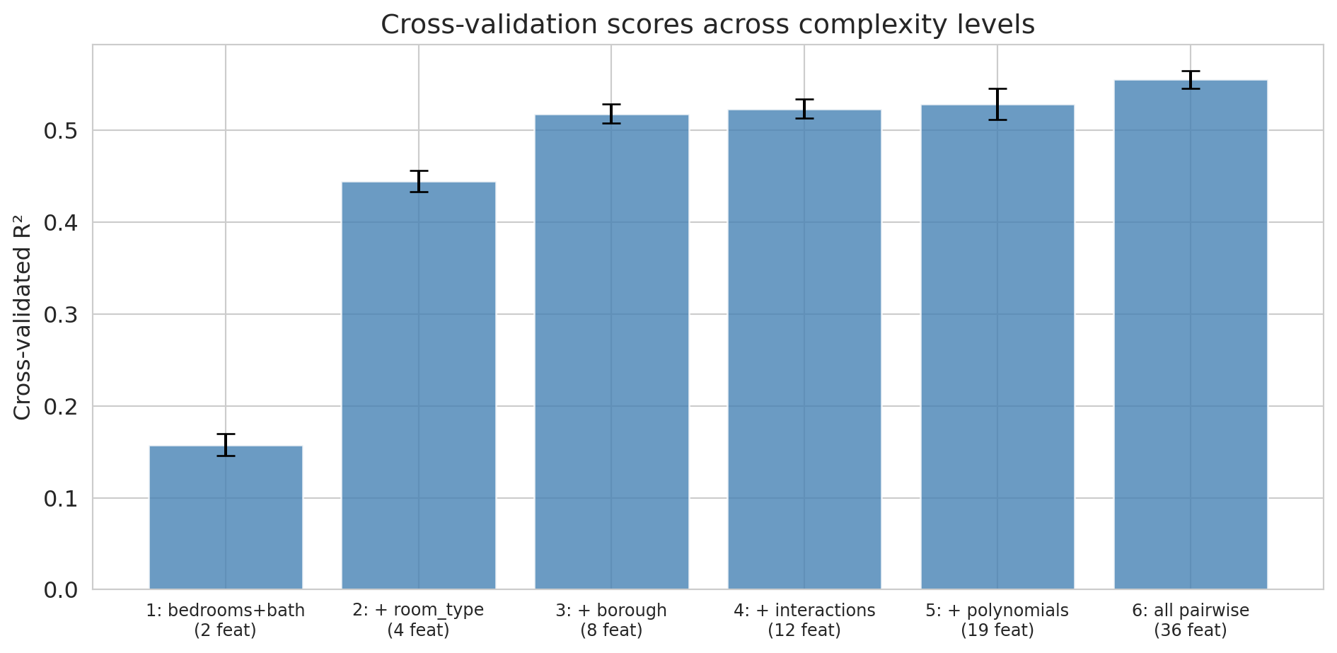
The CV scores give us a more stable comparison than a single train/test split. Let's visualize them with error bars showing the standard deviation across folds.
```{python}
fig, ax = plt.subplots(figsize=(10, 5))
ax.bar(range(len(cv_df)), cv_df['cv_mean'], yerr=cv_df['cv_std'],
       capsize=5, color='steelblue', alpha=0.8, edgecolor='white')
ax.set_xticks(range(len(cv_df)))
ax.set_xticklabels([f'{r["model"]}\n({r["features"]} feat)' for _, r in cv_df.iterrows()],
                   fontsize=9)
ax.set_ylabel('Cross-validated R²')
ax.set_title('Cross-validation scores across complexity levels')
plt.tight_layout()
plt.show()

best = cv_df.loc[cv_df['cv_mean'].idxmax()]
print(f"\nBest model by CV: {best['model']} (CV R² = {best['cv_mean']:.4f})")
```
Cross-validation confirms what the train/test split showed: all six feature sets genuinely help, and the most complex model (Level 6) has the best CV score. With plenty of data relative to the number of features, there's no overfitting to penalize here. Notice that the error bars (standard deviations across folds) give us a sense of how much variability there is — Levels 4 through 6 have overlapping error bars, so the gains from interactions and polynomials are modest. The polynomial experiment above is where CV would earn its keep: it would flag the point where additional polynomial terms start hurting.
:::{.callout-warning}
## CV Assumes Exchangeable Data
CV relies on the assumption that we can shuffle the data randomly — each fold is representative of the whole. The assumption breaks if the data have temporal structure. You can't train on 2024 data and "test" on 2023 data — the model would be peeking into the future. We'll see time-series validation in [Lecture 16](lec16-backtesting.qmd).
:::
## Lasso (regularization)
We've seen two strategies for handling overfitting:
1. **Manually choose** the right number of features using cross-validation
2. But what if we have hundreds of candidate features and don't know which ones matter?
There's a more elegant approach: let the model *automatically* shrink or eliminate unimportant features. That's **Lasso** (Least Absolute Shrinkage and Selection Operator), which adds an L1 penalty to the regression objective:
$$\min_\beta \sum_{i=1}^n (y_i - x_i^T \beta)^2 + \alpha \sum_{j=1}^p |\beta_j|$$
The penalty term $\alpha \sum |\beta_j|$ punishes large coefficients. The key property of L1: it drives some coefficients to *exactly zero*, effectively selecting features automatically.
A close relative is **ridge regression** (L2 regularization), which penalizes $\alpha \sum \beta_j^2$ instead. Ridge shrinks all coefficients toward zero but never sets them exactly to zero — it keeps all features but dampens them. The choice between lasso and ridge depends on whether you believe many features contribute small effects (ridge) or only a few features matter (lasso).
**Practical motivation:** Imagine you're building a medical screening tool. A model that requires 200 blood tests is impractical — it's expensive, slow, and fatiguing for patients. A model that needs 5 blood tests can actually be deployed in a clinic. Lasso finds the parsimonious model automatically.
```{python}
# Small sample to demonstrate overfitting vs. regularization
np.random.seed(42)
df_small = df.sample(500, random_state=42).reset_index(drop=True)
y_small = df_small['price']
train_i, test_i = train_test_split(range(len(df_small)), test_size=0.4, random_state=42)
base_cat = pd.get_dummies(df_small[['room_type', 'borough']], drop_first=True)
X_base_small = pd.concat([df_small[['bedrooms', 'bathrooms']], base_cat], axis=1)

# Use the kitchen-sink polynomial features (degree 3) on the small sample
poly_ks = PolynomialFeatures(degree=3, include_bias=False)
X_ks_small = pd.DataFrame(poly_ks.fit_transform(X_base_small))

X_ks_tr = X_ks_small.iloc[train_i]
X_ks_te = X_ks_small.iloc[test_i]
y_tr = y_small.iloc[train_i]
y_te = y_small.iloc[test_i]

# OLS on the same features (for comparison)
ols_ks = LinearRegression().fit(X_ks_tr, y_tr)

# Lasso automatically shrinks/eliminates features
lasso = Lasso(alpha=1.0, random_state=42).fit(X_ks_tr, y_tr)

n_total = X_ks_small.shape[1]
n_nonzero = (lasso.coef_ != 0).sum()

print(f"Kitchen-sink features: {n_total}")
print(f"Lasso keeps: {n_nonzero} features (zeroed out {n_total - n_nonzero})")
print()
print(f"OLS   — Train R²: {ols_ks.score(X_ks_tr, y_tr):.3f}  Test R²: {r2_score(y_te, ols_ks.predict(X_ks_te)):.3f}")
print(f"Lasso — Train R²: {lasso.score(X_ks_tr, y_tr):.3f}  Test R²: {r2_score(y_te, lasso.predict(X_ks_te)):.3f}")
```
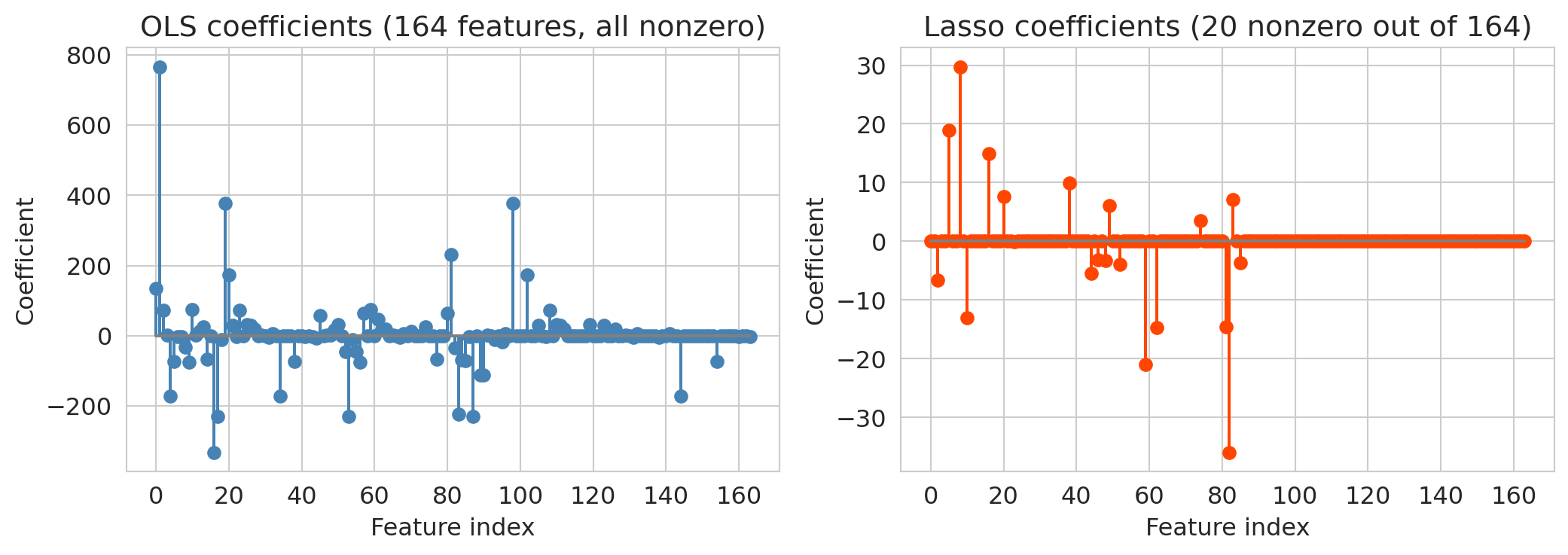
Lasso's test $R^2$ dramatically exceeds OLS on the same features. The coefficient plots below show why: OLS spreads weight across all features (many of which are noise), while `Lasso` zeros most of them out.
```{python}
# Visualize: Lasso coefficients vs OLS coefficients
fig, axes = plt.subplots(1, 2, figsize=(11, 4))

axes[0].stem(range(len(ols_ks.coef_)), ols_ks.coef_, linefmt='steelblue', markerfmt='o', basefmt='gray')
axes[0].set_title(f'OLS coefficients ({n_total} features, all nonzero)')
axes[0].set_xlabel('Feature index')
axes[0].set_ylabel('Coefficient')

axes[1].stem(range(len(lasso.coef_)), lasso.coef_, linefmt='orangered', markerfmt='o', basefmt='gray')
axes[1].set_title(f'Lasso coefficients ({n_nonzero} nonzero out of {n_total})')
axes[1].set_xlabel('Feature index')
axes[1].set_ylabel('Coefficient')

plt.tight_layout()
plt.show()
```
OLS uses all features and overfits more than Lasso — its test $R^2$ (~0.34) is notably worse than Lasso's (~0.48). Lasso aggressively zeros out the noise, keeping only the features that genuinely help prediction. It resolves the overfitting problem automatically: instead of manually choosing how many features to include, let the regularization penalty figure it out.
:::{.callout-tip}
## Think About It
The Lasso penalty strength $\alpha$ controls the bias-variance tradeoff. Large $\alpha$ = more regularization = more features zeroed out = simpler model (higher bias, lower variance). Small $\alpha$ = less regularization = closer to OLS (lower bias, higher variance). You can choose $\alpha$ by cross-validation — as we do next.
:::
### Choosing $\alpha$ by cross-validation
How do we pick the right $\alpha$? Scikit-learn's `LassoCV` automates the search: it fits lasso at many $\alpha$ values, scores each by cross-validation, and selects the $\alpha$ with the best CV performance.
```{python}
# LassoCV searches over a grid of alpha values using 5-fold CV
lasso_cv = LassoCV(cv=5, random_state=42, max_iter=10000).fit(X_ks_tr, y_tr)

print(f"Best alpha: {lasso_cv.alpha_:.4f}")
print(f"Nonzero coefficients: {(lasso_cv.coef_ != 0).sum()} out of {len(lasso_cv.coef_)}")
print(f"Train R²: {lasso_cv.score(X_ks_tr, y_tr):.3f}")
print(f"Test R²:  {r2_score(y_te, lasso_cv.predict(X_ks_te)):.3f}")
```
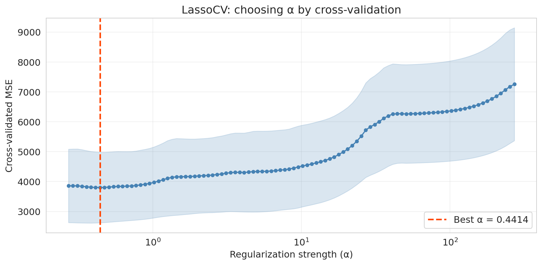
```{python}
# Plot CV error as a function of alpha
fig, ax = plt.subplots(figsize=(10, 5))

# LassoCV stores the mean and std of MSE across folds for each alpha
alphas = lasso_cv.alphas_
mse_mean = lasso_cv.mse_path_.mean(axis=1)
mse_std = lasso_cv.mse_path_.std(axis=1)

ax.plot(alphas, mse_mean, 'o-', color='steelblue', markersize=4)
ax.fill_between(alphas, mse_mean - mse_std, mse_mean + mse_std, alpha=0.2, color='steelblue')
ax.axvline(lasso_cv.alpha_, color='orangered', linestyle='--', linewidth=2,
           label=f'Best α = {lasso_cv.alpha_:.4f}')
ax.set_xscale('log')
ax.set_xlabel('Regularization strength (α)')
ax.set_ylabel('Cross-validated MSE')
ax.set_title('LassoCV: choosing α by cross-validation')
ax.legend(fontsize=12)
ax.grid(True, alpha=0.3)
plt.tight_layout()
plt.show()
```
The U-shaped CV curve confirms the bias-variance tradeoff in action. Too small an $\alpha$ (right side) gives insufficient regularization — the model overfits. Too large an $\alpha$ (left side) penalizes too aggressively — the model underfits. `LassoCV` finds the valley automatically.
## The modern view — averaging overfit trees
The classical story we just told has a satisfying narrative: more complexity eventually leads to overfitting, so we need to regularize. But there's a puzzle.
Random forests use *lots* of parameters — each tree can have thousands of leaves, and we grow hundreds of trees. By the classical logic, they should overfit terribly. But they don't. Why?
### Demo 1: more trees never hurts
Let's train random forests with increasing numbers of trees and track test performance.
```{python}
# Use the full dataset for this demo
X_rf = build_features(df, 3)  # bedrooms, bathrooms, room_type, borough dummies
X_rf_train = build_features(df_train, 3)
X_rf_test = build_features(df_test, 3)

n_trees_list = [1, 5, 10, 25, 50, 100, 200, 500]
rf_test_scores = []

for n_trees in n_trees_list:
    rf = RandomForestRegressor(n_estimators=n_trees, random_state=42, n_jobs=-1)
    rf.fit(X_rf_train, y_train)
    score = rf.score(X_rf_test, y_test)
    rf_test_scores.append(score)
    print(f"n_estimators = {n_trees:>3d}: Test R² = {score:.4f}")
```
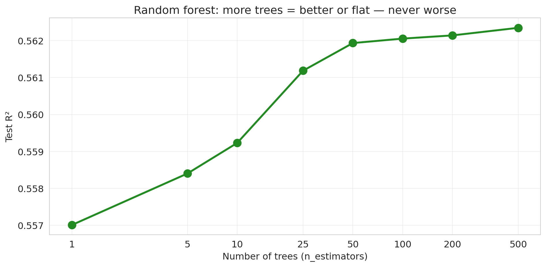
```{python}
fig, ax = plt.subplots(figsize=(10, 5))

ax.plot(n_trees_list, rf_test_scores, 'o-', color='forestgreen', linewidth=2.5, markersize=10)
ax.set_xlabel('Number of trees (n_estimators)')
ax.set_ylabel('Test R²')
ax.set_title('Random forest: more trees = better or flat — never worse')
ax.set_xscale('log')
ax.set_xticks(n_trees_list)
ax.set_xticklabels(n_trees_list)
ax.grid(True, alpha=0.3)
plt.tight_layout()
plt.show()
```
No U-shape! The test $R^2$ increases and then plateaus. Adding more trees never hurts — it just stops helping. The pattern is fundamentally different from the polynomial story, where more complexity eventually *destroyed* test performance. (Caveat: this "more is never worse" property is specific to bagging/random forests. For *gradient boosting*, which we'll meet in Chapter 17, adding too many trees *can* overfit.)
### Demo 2: individual trees are overfit; their average is smooth
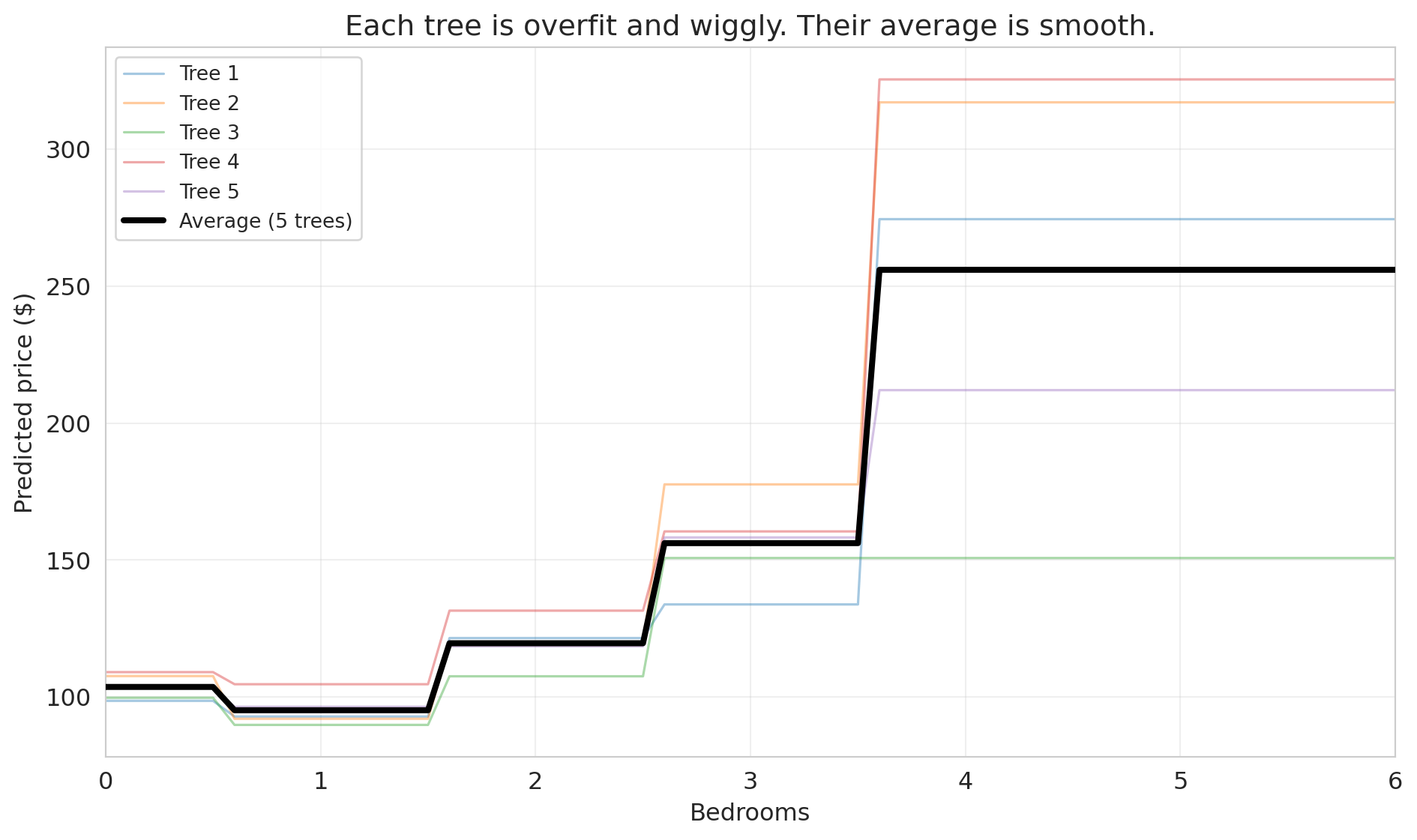
To understand why, let's look at what individual trees actually predict. We'll train 5 decision trees on bootstrap samples and plot their predictions along a 1D slice: price vs. bedrooms, holding other features at their median values.
```{python}
# Create a 1D prediction slice: vary bedrooms, hold everything else at median
median_features = X_rf_train.median()

bedroom_range = np.arange(0, 7, 0.1)
X_slice = pd.DataFrame(
    np.tile(median_features.values, (len(bedroom_range), 1)),
    columns=X_rf_train.columns
)
X_slice['bedrooms'] = bedroom_range

# Train 5 individual trees on bootstrap samples
np.random.seed(42)
fig, ax = plt.subplots(figsize=(10, 6))

individual_preds = []
for i in range(5):
    # Bootstrap sample
    boot_idx = np.random.choice(len(X_rf_train), size=len(X_rf_train), replace=True)
    X_boot = X_rf_train.iloc[boot_idx]
    y_boot = y_train.iloc[boot_idx]

    tree = DecisionTreeRegressor(max_depth=None, random_state=i)
    tree.fit(X_boot, y_boot)
    preds = tree.predict(X_slice)
    individual_preds.append(preds)
    ax.plot(bedroom_range, preds, alpha=0.4, linewidth=1.2, label=f'Tree {i+1}')

# Average prediction
avg_preds = np.mean(individual_preds, axis=0)
ax.plot(bedroom_range, avg_preds, color='black', linewidth=3, label='Average (5 trees)', zorder=5)

ax.set_xlabel('Bedrooms')
ax.set_ylabel('Predicted price ($)')
ax.set_title('Each tree is overfit and wiggly. Their average is smooth.')
ax.legend(fontsize=10, loc='upper left')
ax.set_xlim(0, 6)
ax.grid(True, alpha=0.3)
plt.tight_layout()
plt.show()
```
Each individual tree (thin colored lines) is wiggly and overfit — it has memorized the quirks of its particular bootstrap sample. But their *errors point in different directions*. One tree might predict too high for 3-bedroom listings while another predicts too low. When we average them, the noise cancels out, and what remains is the genuine signal.
The core insight of **bagging** (bootstrap aggregating): averaging many overfit models reduces variance without increasing bias. It's the same principle behind asking 100 people to estimate the weight of a cow at a county fair — individual guesses vary wildly, but the average is remarkably accurate.
One sentence looking ahead: this same principle — overparameterize, then regularize implicitly through averaging — is part of why large language models work. We'll revisit this connection in [Lecture 17](lec17-automl-llms.qmd).
**The upshot:** the classical advice "regularize and cross-validate" still works. But now you know there's another path: build many diverse models and average them. The bias-variance tradeoff isn't wrong — it's just not the whole story.
### How trees handle missing data
Unlike linear regression, which requires complete data for every row, decision trees can handle missing values directly. Different implementations use different strategies:
**Surrogate splits.** When a tree encounters a missing value at a split node, it looks for an alternative feature that produces a similar partition. If the best split is on `bedrooms` and a row has a missing bedroom count, the tree might split on `accommodates` instead (a correlated feature). CART and scikit-learn's `DecisionTreeClassifier` use this approach.
**Native missing-value handling.** XGBoost and LightGBM go further: during training, they learn which branch (left or right) missing values should follow at each split, choosing whichever direction reduces the loss more. No imputation needed — the algorithm treats "missing" as just another value to route.
**Why trees handle this well.** A decision tree asks a yes/no question at each node. Missing values simply need a rule for which branch to follow. Linear models, by contrast, need a numeric value to multiply by a coefficient — a missing value breaks the computation entirely.
:::{.callout-tip}
## Think About It
If 30% of your `bedrooms` column is missing and you impute with the median before fitting a tree, what information have you destroyed? Would the tree have been better off seeing the missingness directly?
:::
In practice, tree-based models (especially gradient-boosted trees like XGBoost) are the most popular choice for tabular data with missing values — precisely because they don't require the analyst to make imputation decisions that could introduce bias.
## Key takeaways
- **Always evaluate on held-out data.** Training $R^2$ is a measure of memory, not understanding. A model that memorizes the training set perfectly can fail catastrophically on new data.
- **Cross-validation for stable model comparison.** A single train/test split is noisy. CV rotates which fold is held out and averages the results, giving a reliable estimate of out-of-sample performance.
- **Bias-variance tradeoff: the classical U-shape.** Too simple (high bias, underfitting) is bad. Too complex (high variance, overfitting) is bad. Expected test error = bias$^2$ + variance + $\sigma^2$, where $\sigma^2$ is irreducible noise. The goal is to minimize the first two terms.
- **Lasso: automatic feature selection via regularization.** Instead of manually choosing features, let the L1 penalty shrink unimportant coefficients to exactly zero.
- **Modern view: averaging overfit trees reduces variance — no U-shape for `n_estimators`.** Each tree is overfit, but their errors point in different directions. Averaging cancels noise without losing signal.
- **Forward references:** [Lecture 8](lec08-sampling.qmd) (bootstrap — can we trust our estimates?), [Lecture 12](lec12-regression-inference.qmd) (regression inference — which features are statistically significant?), [Lecture 16](lec16-backtesting.qmd) (temporal validation — why CV breaks for time series), [Lecture 17](lec17-automl-llms.qmd) (trees deep dive — how random forests actually work).
## Study guide
### Key ideas
- **Train/test split** — holding out part of the data to evaluate model performance on unseen data.
- **Validation set** — data used to choose model complexity (distinct from the final test set).
- **Cross-validation (k-fold)** — rotating which of $k$ folds is held out, averaging test scores for a more stable estimate of out-of-sample performance.
- **Overfitting** — the model memorizes training data (including noise) and performs poorly on new data. Training $R^2$ always improves with more features; when features outnumber effective data points, test $R^2$ can degrade dramatically — the gap between train and test performance is overfitting.
- **Underfitting** — the model is too simple to capture the real pattern in the data.
- **Bias-variance tradeoff** — the tension between underfitting (high bias) and overfitting (high variance). For MSE: expected test error = bias$^2$ + variance + $\sigma^2$ (irreducible noise). The goal is to minimize the first two terms; $\sigma^2$ sets the floor.
- **Lasso (L1 regularization)** — adds a penalty $\alpha \sum |\beta_j|$ that shrinks some coefficients to exactly zero, performing automatic feature selection.
- **Ridge (L2 regularization)** — adds a penalty $\alpha \sum \beta_j^2$ that shrinks coefficients toward zero but does not set them exactly to zero; useful when many features contribute small effects.
- **Regularization** — constraining model complexity to reduce overfitting. Lasso and ridge are the two main forms for linear regression.
- **Bagging** — bootstrap aggregating: training many models on bootstrap samples and averaging their predictions to reduce variance. More trees never hurts.
- **Leave-one-out CV (LOO-CV)** — the extreme case of $k$-fold CV where $k = n$; each observation gets its own fold. Low bias but high variance and computationally expensive.
- **Irreducible noise ($\sigma^2$)** — inherent randomness in the outcome that no model can eliminate. Even the true model faces this floor on test error.
- **Three-way split (train / validation / test)** — training data for fitting, validation data for choosing model complexity, test data for final evaluation. Using the test set for model selection contaminates the performance estimate.
- **Trees and missing data** — tree-based models handle missing data natively — by learning surrogate splits or optimal missing-value routing. Linear models require complete data or explicit imputation.
### Computational tools
- `train_test_split(X, y, test_size=0.3)` — splits data into training and test sets
- `cross_val_score(model, X, y, cv=5)` — performs 5-fold cross-validation and returns scores per fold
- `Lasso(alpha=1.0).fit(X, y)` — fits a Lasso regression with regularization strength `alpha`
- `LassoCV(cv=5).fit(X, y)` — searches over `alpha` values by cross-validation, selects the best
- `RandomForestRegressor(n_estimators=100).fit(X, y)` — fits a random forest; more trees = better or flat, never worse
- `xgboost.XGBRegressor()` / `lightgbm.LGBMRegressor()` — gradient-boosted tree libraries that handle missing values natively (no imputation required)
### For the quiz
You are responsible for: train/test split, cross-validation (how it works and why it's better than a single split), overfitting concept, bias-variance tradeoff (the classical U-shape), Lasso concept (what it does, not the optimization details), and why random forest test error plateaus rather than showing a U-shape.