---
title: "Linear Regression as Projection"
execute:
enabled: true
jupyter: python3
---
```{python}
import numpy as np
import pandas as pd
import matplotlib.pyplot as plt
import seaborn as sns
from sklearn.linear_model import LinearRegression
from mpl_toolkits.mplot3d import Axes3D
import warnings
warnings.filterwarnings('ignore')
sns.set_style('whitegrid')
plt.rcParams['figure.figsize'] = (7, 4.5)
plt.rcParams['font.size'] = 12

# Load data
DATA_DIR = 'data'
```
## How much is a bathroom worth?
An Airbnb host adds a second bathroom. How much more should they charge per night?
Regression gives the answer — and linear algebra tells us **why** it works.
You may have *used* the regression formula before. This chapter develops the geometric view — essential when we add many features, diagnose problems, and eventually ask causal questions. The central idea: regression is a **projection**.
## The data
Let's load the NYC Airbnb dataset and focus on listings with reasonable prices.
```{python}
# Load and clean Airbnb data
airbnb = pd.read_csv(f'{DATA_DIR}/airbnb/listings.csv', low_memory=False)

# Parse price (handles both "$1,200.00" strings and numeric formats)
airbnb['price_clean'] = (airbnb['price'].astype(str)
                          .str.replace('[$,]', '', regex=True)
                          .astype(float))

# Working subset
cols = ['bedrooms', 'bathrooms', 'beds', 'price_clean',
        'accommodates', 'number_of_reviews', 'room_type']
df = airbnb[cols].dropna()  # drops rows with missing bedrooms, bathrooms, etc.
df = df[(df['price_clean'] > 0) & (df['price_clean'] <= 500)]
print(f"{len(df):,} listings, price range: ${df['price_clean'].min():.0f} – ${df['price_clean'].max():.0f}")
df.head()
```
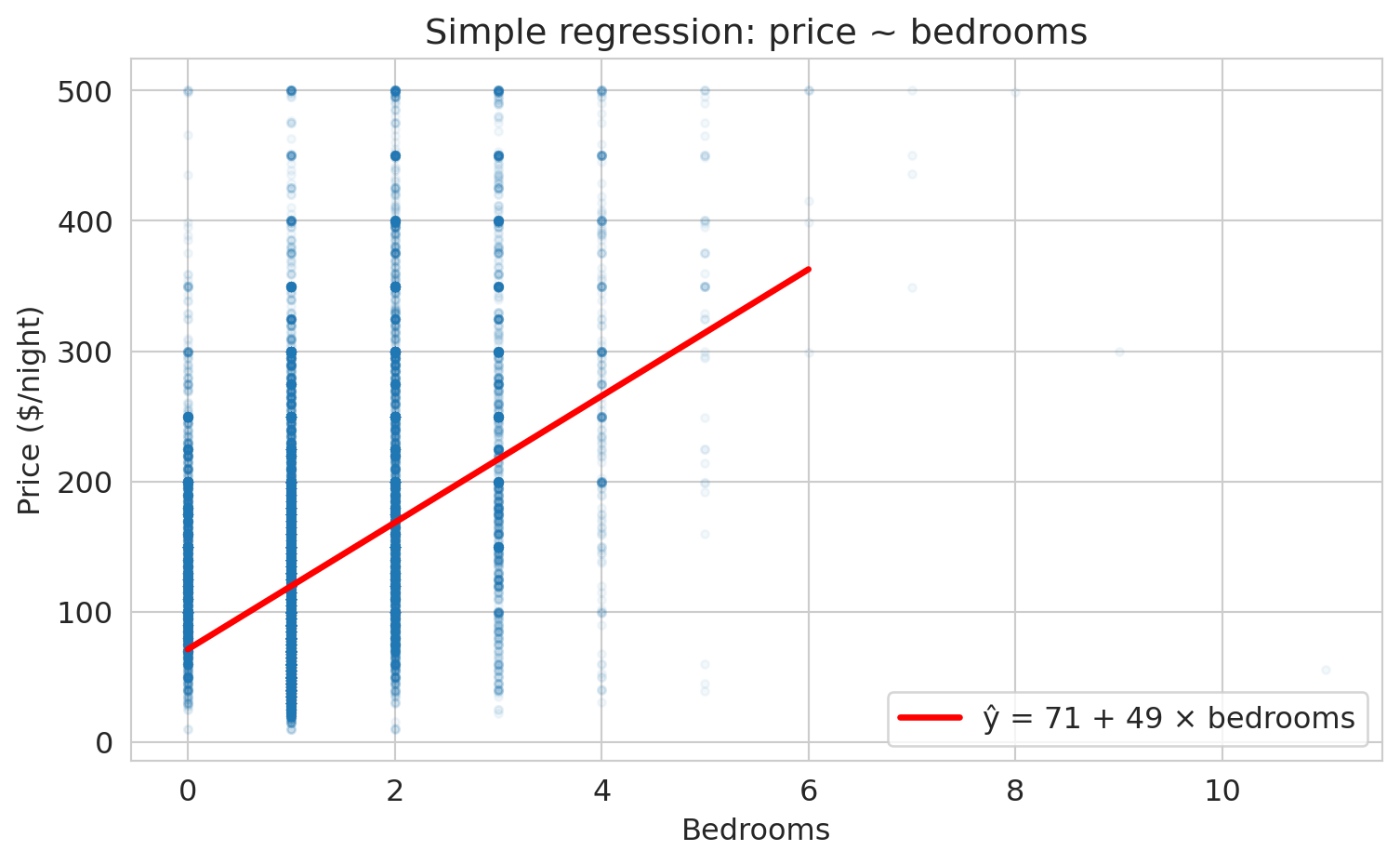
## Simple regression: price ~ bedrooms
Let's start simple. How does price change with the number of bedrooms?
```{python}
# Scatter plot + regression line
fig, ax = plt.subplots(figsize=(8, 5))
ax.scatter(df['bedrooms'], df['price_clean'], alpha=0.05, s=10)

# Fit simple regression
model_simple = LinearRegression()
model_simple.fit(df[['bedrooms']], df['price_clean'])
x_line = np.linspace(0, 6, 100)
y_line = model_simple.predict(x_line.reshape(-1, 1))
ax.plot(x_line, y_line, 'r-', lw=2.5, label=f'ŷ = {model_simple.intercept_:.0f} + {model_simple.coef_[0]:.0f} × bedrooms')

ax.set_xlabel('Bedrooms')
ax.set_ylabel('Price ($/night)')
ax.set_title('Simple regression: price ~ bedrooms')
ax.legend(fontsize=12)
plt.tight_layout()
plt.show()

print(f"Each additional bedroom is associated with ${model_simple.coef_[0]:.0f} more per night.")
```
:::{.callout-note}
## Why is it called "regression"?
The name comes from Francis Galton, who in the 1880s studied the heights of fathers and sons. Unusually tall fathers tended to have sons who were tall — but *less* tall than their fathers. Unusually short fathers had sons who were short — but *less* short. Heights "regressed toward the mean." Galton's method for quantifying this trend — fitting a line through the data — became "regression," and the name stuck even though we now use it for problems that have nothing to do with reverting to averages. We will formalize **regression to the mean** shortly, once we connect $r$ to $R^2$. (For the full story, see Salsburg, *The Lady Tasting Tea*, Ch. 4.)
:::
That's the regression line. But *why* this line? There are infinitely many lines we could draw through this cloud. Regression picks the one that minimizes the total squared distance from the data to the line. Why squared distances, not absolute distances or something else?
:::{.callout-tip}
## Think About It
Why minimize *squared* errors? Two reasons: (1) squared error leads to a linear algebra problem — the projection — with a clean closed-form solution; (2) it estimates the conditional mean. We could choose a different loss function (and we will, in Chapter 13 for classification). For now, squared error gives us the most elegant geometry.
:::
## The geometric view: prediction lives in the column space
Here's the key idea from Chapter 4:
- Your feature matrix $X$ has columns $x_1, x_2, \ldots$
- Any prediction $\hat{y} = X\beta$ is a **linear combination** of those columns
- So $\hat{y}$ must live in the **column space** of $X$
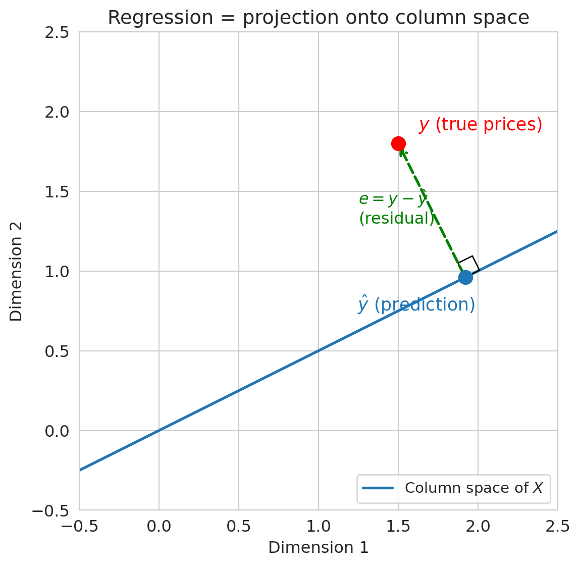
The true prices $y$ probably do NOT live in the column space. So regression finds the **closest point** in the column space to $y$. That closest point is the **projection** of $y$ onto $\text{col}(X)$.
As George Box put it: **"All models are wrong, but some are useful."** The prediction $\hat{y}$ won't equal $y$ exactly — the model is wrong — but projection gives us the *best approximation* within the column space.
:::{.callout-tip}
## Think About It
If $\hat{y}$ is the closest point in the column space to $y$, what direction must $y - \hat{y}$ point? (Hint: think about the closest point on a line to a point not on the line.)
:::
```{python}
# Visualization code — focus on the output, not the plotting details.
# This draws a 2D cartoon: y is a point, col(X) is a line,
# and ŷ is the projection of y onto that line.

fig, ax = plt.subplots(figsize=(7, 6))

# The column space (a line through the origin in this picture)
t = np.linspace(-0.5, 2.5, 100)
ax.plot(t, 0.5 * t, 'C0-', lw=2, label='Column space of $X$')

# y (the target)
y_pt = np.array([1.5, 1.8])
ax.plot(*y_pt, 'ro', ms=10, zorder=5)
ax.annotate('$y$ (true prices)', xy=y_pt, fontsize=13,
            xytext=(15, 10), textcoords='offset points', color='red')

# ŷ (the projection)
# Project y onto the line (direction [1, 0.5])
d = np.array([1, 0.5])
d_unit = d / np.linalg.norm(d)
yhat_pt = np.dot(y_pt, d_unit) * d_unit
ax.plot(*yhat_pt, 'C0o', ms=10, zorder=5)
ax.annotate('$\hat{y}$ (prediction)', xy=yhat_pt, fontsize=13,
            xytext=(-80, -25), textcoords='offset points', color='C0')

# Residual (orthogonal)
ax.annotate('', xy=y_pt, xytext=yhat_pt,
            arrowprops=dict(arrowstyle='->', color='green', lw=2, ls='--'))
ax.text(1.25, 1.3, '$e = y - \hat{y}$\n(residual)', fontsize=12, color='green')

# Right angle marker
from matplotlib.patches import Rectangle
angle_size = 0.1
corner = yhat_pt
perp = (y_pt - yhat_pt)
perp_unit = perp / np.linalg.norm(perp)
par_unit = d_unit
sq = np.array([corner, corner + angle_size*par_unit,
               corner + angle_size*par_unit + angle_size*perp_unit,
               corner + angle_size*perp_unit, corner])
ax.plot(sq[:, 0], sq[:, 1], 'k-', lw=1)

ax.set_xlim(-0.5, 2.5)
ax.set_ylim(-0.5, 2.5)
ax.set_aspect('equal')
ax.set_xlabel('Dimension 1')
ax.set_ylabel('Dimension 2')
ax.set_title('Regression = projection onto column space')
ax.legend(loc='lower right', fontsize=11)
plt.tight_layout()
plt.show()
```
The **residual** $e = y - \hat{y}$ is **orthogonal** to the column space. Orthogonality is the defining property of the least squares solution.
Why orthogonal? The perpendicular from a point to a subspace gives the closest point — just as dropping a perpendicular from a point to a line gives the nearest point on the line.
## Normal equations: orthogonality in algebra
We're about to derive a formula for the regression coefficients that explains WHY sklearn gives the answer it does. The key insight: requiring the residual to be orthogonal to $X$ gives us exactly one equation to solve.
"The residual is orthogonal to the column space" translates to:
$$X^T(y - X\beta) = 0$$
The condition states that the residual $e = y - X\beta$ has zero dot product with every column of $X$. Rearranging:
$$X^T X \beta = X^T y \qquad \Longrightarrow \qquad \beta = (X^T X)^{-1} X^T y$$
:::{.callout-important}
## Definition: Normal Equations
The **normal equations** $X^TX\beta = X^Ty$ give the least squares solution $\beta = (X^TX)^{-1}X^Ty$. The formula requires $X^TX$ to be invertible, which means the columns of $X$ must be linearly independent (recall Chapter 4). Perfectly collinear features make the matrix singular, so no unique solution exists.
:::
You may have heard "regression minimizes the sum of squared errors." Now you can see *why*: the prediction that minimizes $\|y - \hat{y}\|^2$ is exactly the orthogonal projection of $y$ onto $\text{col}(X)$.
The normal equations give us the exact solution in one step. For larger problems or different loss functions where no closed-form solution exists, we'll need an iterative approach called gradient descent (Chapter 13).
```{python}
# Verify: the normal equations give the same answer as sklearn

# Simple regression with an intercept: price = beta0 + beta1 * bedrooms
X_bedrooms = np.column_stack([np.ones(len(df)), df['bedrooms'].values])
prices = df['price_clean'].values

# Normal equations: beta = (X^T X)^{-1} X^T y
# We use np.linalg.solve rather than np.linalg.inv — computing matrix
# inverses explicitly is numerically unstable. For even better numerical
# stability, production code uses the QR factorization (VMLS Ch 13).
beta_normal = np.linalg.solve(X_bedrooms.T @ X_bedrooms, X_bedrooms.T @ prices)

print("Normal equations:  intercept = {:.2f}, slope = {:.2f}".format(*beta_normal))
print("sklearn:           intercept = {:.2f}, slope = {:.2f}".format(
    model_simple.intercept_, model_simple.coef_[0]))
```
The two solutions match. Now let's verify the orthogonality property directly: the residuals should have zero dot product with every column of $X$.
```{python}
# Verify orthogonality: residuals are orthogonal to each column of X
prices_hat = X_bedrooms @ beta_normal
residuals = prices - prices_hat

dot_with_ones = np.dot(residuals, X_bedrooms[:, 0])     # dot with intercept column
dot_with_bedrooms = np.dot(residuals, X_bedrooms[:, 1])  # dot with bedrooms column

print("Residuals dot (column of 1s):  {:.6f}  (≈ 0 ✓)".format(dot_with_ones))
print("Residuals dot (bedrooms):      {:.6f}  (≈ 0 ✓)".format(dot_with_bedrooms))
print()
print("The residual is orthogonal to every column of X.")
print("This IS the normal equation: X^T(y - Xβ) = 0.")
print("The errors have no pattern left that could be captured by the features.")
```
## From correlation to $R^2$
Before adding more features, let's connect the simple regression we just ran to a quantity you've seen in introductory statistics: the **correlation coefficient** $r$.
The correlation coefficient $r$ measures the strength and direction of the linear association between two variables. It ranges from $-1$ (perfect negative linear relationship) to $+1$ (perfect positive). In the Data 8 formulation, the regression line can be written as $\hat{y} = r \cdot \frac{SD_y}{SD_x}(x - \bar{x}) + \bar{y}$, which makes $r$ the slope in standardized units.
```{python}
# Compute the correlation coefficient between price and bedrooms
r = df['price_clean'].corr(df['bedrooms'])
print(f"Correlation between price and bedrooms: r = {r:.4f}")
print(f"r² = {r**2:.4f}")
print()

# Compare to R² from the simple regression
y_hat_simple = model_simple.predict(df[['bedrooms']])
ss_res = np.sum((df['price_clean'] - y_hat_simple)**2)
ss_tot = np.sum((df['price_clean'] - df['price_clean'].mean())**2)
r2_simple_model = 1 - ss_res / ss_tot
print(f"R² from simple regression: {r2_simple_model:.4f}")
print(f"They match: r² = R² in simple regression.")
```
:::{.callout-important}
## $R^2 = r^2$ in simple regression
For a model with **one** predictor, $R^2$ is literally the square of the correlation coefficient $r$. The distinction matters: $r$ and $R^2$ are different quantities that happen to be related by squaring in the simple case. With multiple predictors, $R^2$ still measures the fraction of variance explained, but there's no single $r$ to square.
:::
The connection between $r$ and $R^2$ also explains Galton's original observation. For real data, $|r| < 1$, so the predicted value $\hat{y}$ is always *closer to the mean* than $x$ is (in standardized units). Fathers who are 2 SDs above average height have sons whose predicted height is only $r \times 2$ SDs above average — less extreme, pulled back toward the mean.
:::{.callout-important}
## Definition: Regression to the mean
**Regression to the mean** is the phenomenon whereby extreme observations tend to be followed by less extreme ones. It arises whenever the correlation between successive measurements is imperfect ($|r| < 1$) and is a purely statistical phenomenon — not a biological or physical one. Galton's observation of heights "regressing" toward the average is the origin of the term "regression" itself.
:::
## Multiple regression: more features, bigger column space
Our model says each bedroom adds some amount per night. But bigger apartments also have more bathrooms and can accommodate more guests. The bedroom coefficient might be picking up the effect of all of these correlated features. To isolate the bedroom effect, we need to *hold other features constant*.
Each new (independent) feature expands the column space, giving us a richer set of possible predictions.
Think of regression as having two choices: (1) the column space — which features to include, determining what predictions the model can make — and (2) the loss function — squared error, which gives us the projection. Change the features and you change what the model can express. Change the loss and you change what "best" means. We'll explore both directions in later lectures.
```{python}
# Multiple regression: price ~ bedrooms + bathrooms + room_type
# One-hot encode room_type
df_model = df.copy()
df_model = pd.get_dummies(df_model, columns=['room_type'], drop_first=True, dtype=float)

features = ['bedrooms', 'bathrooms', 'room_type_Private room', 'room_type_Shared room']
X_multi = df_model[features]
y_multi = df_model['price_clean']

model_multi = LinearRegression()
model_multi.fit(X_multi, y_multi)

print("Multiple regression: price ~ bedrooms + bathrooms + room_type")
print(f"  Intercept: ${model_multi.intercept_:.2f}")
print()
for feat, coef in zip(features, model_multi.coef_):
    print(f"  {feat:30s}  ${coef:+.2f}")
```
**Coefficient interpretation:**
- Each additional bedroom is associated with about \$33 more per night, **holding other features constant**.
- Each additional bathroom is associated with about \$22 more per night.
- A private room costs roughly \$90 *less* than an entire home/apt, all else equal.
Now we can answer the opening question: our host should charge about \$22 more for that second bathroom, holding bedrooms and room type fixed.
The "holding constant" part is crucial — multiple regression provides something simple regression cannot. The coefficient on bedrooms means that if we compare two listings with the same number of bathrooms, the same room type, and the same everything else — but one has one more bedroom — the model predicts the extra bedroom is worth about \$33/night.
These coefficients are **point estimates** — we'll quantify their uncertainty with confidence intervals in Chapter 12.
We can go even further: adding polynomial features, interactions, or other transformations expands the column space without leaving the linear regression framework. We'll explore this expansion in Chapter 6.
```{python}
# Compare simple vs multiple regression
model_bed_only = LinearRegression().fit(df[['bedrooms']], df['price_clean'])
y_hat_simple = model_bed_only.predict(df[['bedrooms']])
y_hat_multi = model_multi.predict(X_multi)

r2_simple = 1 - np.sum((y_multi - y_hat_simple)**2) / np.sum((y_multi - y_multi.mean())**2)
r2_multi = 1 - np.sum((y_multi - y_hat_multi)**2) / np.sum((y_multi - y_multi.mean())**2)

print(f"R² with bedrooms only:                          {r2_simple:.3f}")
print(f"R² with bedrooms + bathrooms + room_type:        {r2_multi:.3f}")
print()
print("More independent features → larger column space → better projection → higher R²")
```
## $R^2$ as a projection ratio
After centering $y$ (subtracting the mean), we can decompose:
$$\|y - \bar{y}\|^2 = \|\hat{y} - \bar{y}\|^2 + \|e\|^2$$
The right-hand side is a Pythagorean decomposition — $\hat{y} - \bar{y}$ and $e$ are orthogonal. The equality holds when the model includes an intercept (which ours does); the intercept ensures residuals sum to zero via the normal equation $\mathbf{1}^T e = 0$.
$$R^2 = \frac{\|\hat{y} - \bar{y}\|^2}{\|y - \bar{y}\|^2} = 1 - \frac{\|e\|^2}{\|y - \bar{y}\|^2}$$
:::{.callout-important}
## Definition: $R^2$
$R^2$ is the fraction of variance "explained" — geometrically, it's the squared cosine of the angle $\theta$ between the centered response $y - \bar{y}$ and the centered predictions $\hat{y} - \bar{y}$. The Pythagorean decomposition above is precisely $1 = \cos^2\theta + \sin^2\theta$, so $R^2 = \cos^2\theta$.
:::
```{python}
# Verify the Pythagorean decomposition
y_vals = y_multi.values
y_bar = y_vals.mean()
y_hat_vals = y_hat_multi

ss_total = np.sum((y_vals - y_bar)**2)        # ||y - ȳ||²
ss_model = np.sum((y_hat_vals - y_bar)**2)    # ||ŷ - ȳ||²
ss_resid = np.sum((y_vals - y_hat_vals)**2)   # ||e||²

print(f"SS_total = {ss_total:,.0f}")
print(f"SS_model = {ss_model:,.0f}")
print(f"SS_resid = {ss_resid:,.0f}")
print(f"SS_model + SS_resid = {ss_model + ss_resid:,.0f}  (≈ SS_total ✓)")
print()
print(f"R² = SS_model / SS_total = {ss_model/ss_total:.4f}")
print(f"R² = 1 - SS_resid/SS_total = {1 - ss_resid/ss_total:.4f}")
```
An $R^2$ around 0.45 means our model explains about 45% of the variation in prices. The remaining 55% comes from factors we didn't include — neighborhood, amenities, photos, host reputation.
:::{.callout-tip}
## Think About It
Can R-squared ever *decrease* when you add a feature? Why or why not? (We'll answer this in a moment.)
:::
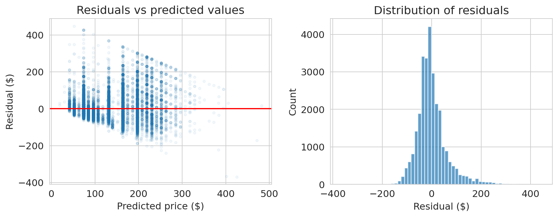
## Checking the residuals
The normal equations guarantee $X^Te = 0$ — that's a mathematical fact. But a good model should also have residuals that look like random noise. The orthogonality is guaranteed; the randomness is not. Let's check.
```{python}
# Residual plot
residuals_multi = y_multi - y_hat_multi

fig, axes = plt.subplots(1, 2, figsize=(10, 4))

axes[0].scatter(y_hat_multi, residuals_multi, alpha=0.05, s=10)
axes[0].axhline(0, color='red', lw=1.5)
axes[0].set_xlabel('Predicted price ($)')
axes[0].set_ylabel('Residual ($)')
axes[0].set_title('Residuals vs predicted values')

axes[1].hist(residuals_multi, bins=60, edgecolor='white', alpha=0.7)
axes[1].set_xlabel('Residual ($)')
axes[1].set_ylabel('Count')
axes[1].set_title('Distribution of residuals')

plt.tight_layout()
plt.show()

print("Notice: the spread of residuals increases with predicted price.")
print("This is heteroscedasticity — the model's errors are not constant.")
```
:::{.callout-warning}
## Heteroscedasticity
When the spread of residuals changes with the predicted value, we have **heteroscedasticity**. Coefficient estimates remain valid, but standard errors from the usual OLS formula become unreliable under heteroscedasticity. We'll revisit this issue in Chapter 12.
:::
## Does popularity cause higher prices?
Let's add `number_of_reviews` as a feature. More reviews might mean a listing is more popular. Does that predict higher prices?
```{python}
# Add number_of_reviews to the model
features_plus = features + ['number_of_reviews']
X_plus = df_model[features_plus]

model_plus = LinearRegression()
model_plus.fit(X_plus, y_multi)

y_hat_plus = model_plus.predict(X_plus)
r2_plus = 1 - np.sum((y_multi - y_hat_plus)**2) / np.sum((y_multi - y_multi.mean())**2)

print("Model with number_of_reviews added:")
print(f"  R² = {r2_plus:.4f}  (was {r2_multi:.4f})")
print()
for feat, coef in zip(features_plus, model_plus.coef_):
    print(f"  {feat:30s}  ${coef:+.2f}")
```
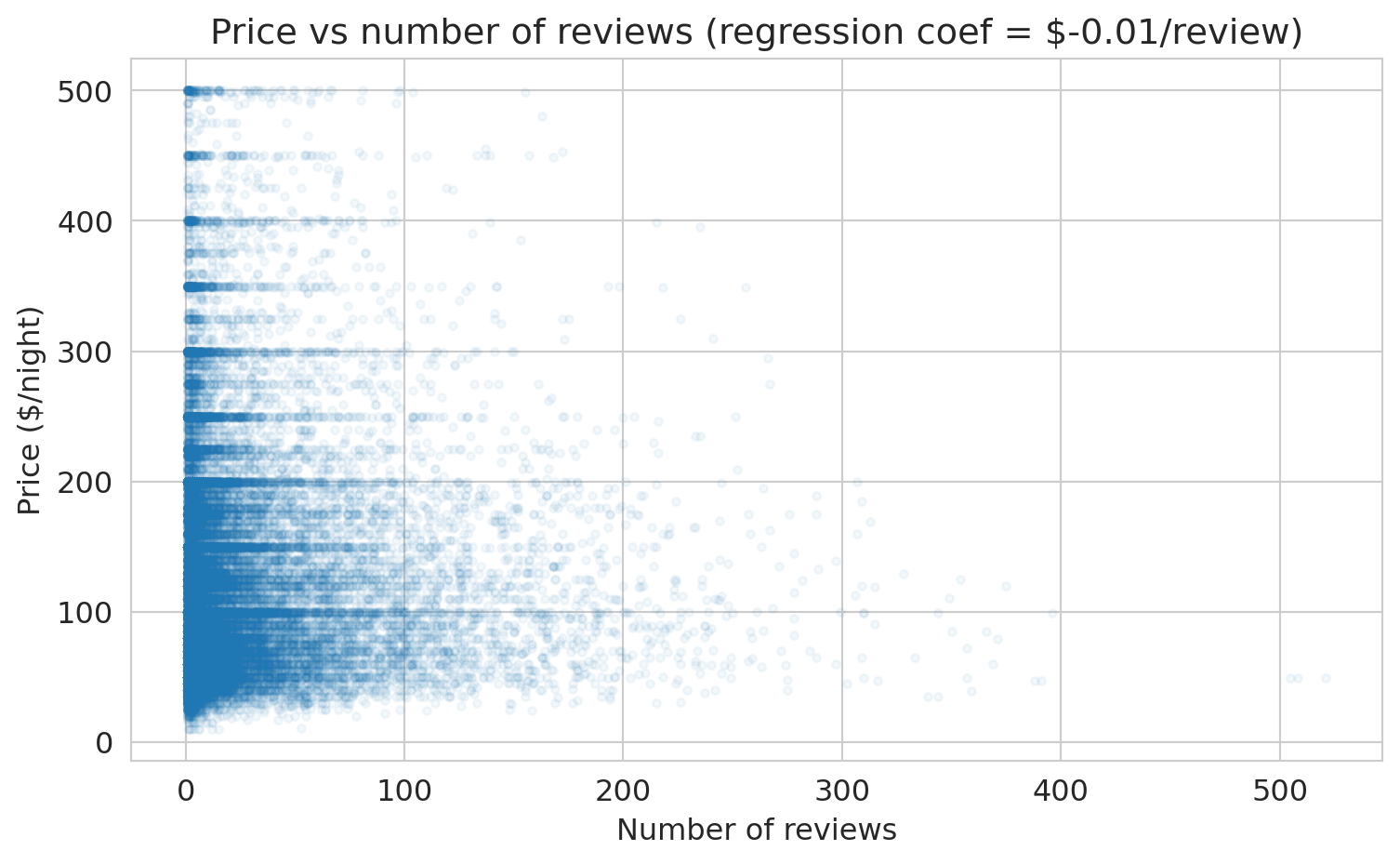
The coefficient on `number_of_reviews` is negative. Let's visualize the relationship directly.
```{python}
# The coefficient on number_of_reviews
coef_reviews = model_plus.coef_[-1]

fig, ax = plt.subplots(figsize=(8, 5))
ax.scatter(df['number_of_reviews'], df['price_clean'], alpha=0.05, s=10)
ax.set_xlabel('Number of reviews')
ax.set_ylabel('Price ($/night)')
ax.set_title(f'Price vs number of reviews (regression coef = ${coef_reviews:.2f}/review)')
plt.tight_layout()
plt.show()

print(f"The coefficient is ${coef_reviews:.2f} per review.")
print("Listings with MORE reviews tend to be slightly CHEAPER.")
print()
print("Wait — does getting more reviews CAUSE a listing to be cheaper?")
print("Of course not. This is correlation, not causation.")
print("Cheaper listings get booked more → more reviews.")
print("We'll revisit this when we study causal inference.")
```
**Training** $R^2$ remained essentially unchanged when we added `number_of_reviews` — it barely moved the projection closer to $y$. **Training $R^2$ can NEVER decrease when you add a feature** — that's a mathematical fact about projections (a bigger column space means a closer projection). But this doesn't mean the model is better at predicting *new* data. We'll see this distinction clearly in Chapter 7.
:::{.callout-warning}
## Correlation is not causation
Does `number_of_reviews` *cause* higher or lower prices? No. A \$50/night studio in Manhattan gets booked 200 nights a year. A \$400/night penthouse gets booked 30 nights a year. More bookings means more guests means more reviews. Price drives both bookings and review count. The pattern illustrates **confounding** — a hidden common cause creates a misleading association. We'll formalize confounding with DAGs in Chapter 18.
:::
:::{.callout-tip}
## Think About It
If you wanted to know whether adding a bathroom *causes* a price increase, how would you design a study? (We'll answer this in the causal inference lectures.)
:::
## Preview: does more features = better predictions?
Training $R^2$ always goes up with more features. But what about predictions on *new* data? A quick **train/test split** reveals the distinction.
```{python}
# Split data: train on 80%, test on 20%
from sklearn.model_selection import train_test_split

train, test = train_test_split(df_model, test_size=0.2, random_state=42)

features_small = ['bedrooms']
features_big = features_plus  # bedrooms + bathrooms + room_type + number_of_reviews

model_small = LinearRegression().fit(train[features_small], train['price_clean'])
model_big = LinearRegression().fit(train[features_big], train['price_clean'])

for name, mod, feats in [("bedrooms only", model_small, features_small),
                          ("all features", model_big, features_big)]:
    r2_train = mod.score(train[feats], train['price_clean'])
    r2_test = mod.score(test[feats], test['price_clean'])
    print(f"{name:20s}  train R² = {r2_train:.4f},  test R² = {r2_test:.4f}")
```
Training $R^2$ goes up with more features — guaranteed. Test $R^2$ *usually* goes up too, but not always, and not by as much. A large gap between train and test $R^2$ signals **overfitting** — the model fits noise in the training data that doesn't generalize. We'll develop train/test splitting properly in Chapter 7.
## Key takeaways
- **Regression is projection.** The prediction $\hat{y}$ is the orthogonal projection of $y$ onto the column space of $X$.
- **The residual is orthogonal to the column space:** $X^Te = 0$. Orthogonality IS the normal equation.
- **The normal equations** $\beta = (X^TX)^{-1}X^Ty$ give the least squares solution (when $X^TX$ is invertible). Now you know *why* it works.
- **$R^2$** is the fraction of variance explained — the squared cosine between $y - \bar{y}$ and $\hat{y} - \bar{y}$.
- **More features → higher training $R^2$**, guaranteed. But higher training $R^2$ does NOT mean better predictions on new data or causal understanding.
- Regression finds the **best approximation** to $y$ in the column space of $X$. "All models are wrong, but some are useful" (Box).
Next: can we make this model more powerful? With the right features — dummies, polynomials, interactions — a linear model can capture surprisingly complex patterns. And we'll meet decision trees, which engineer features automatically. (Chapter 6: Feature Engineering.)
## Connections
- **EE103/CME103 (VMLS):** The material here is least squares from Ch 13, applied to real data.
- **ORIE 4741 framing:** We chose a model family (linear functions) and a loss (squared error). The normal equations solve the optimization problem. ORIE 4741 solves this same problem via gradient descent — a different route to the same answer.
- **Coming up:** Feature engineering — polynomials, interactions, trees (Chapter 6), validation and the bias-variance tradeoff (Chapter 7), bootstrap CIs (Chapter 8), regression diagnostics and inference (Chapter 12), and eventually: when does correlation imply causation? (Chapters 18–19).
## Study guide
### Key ideas
- **Projection** — the closest point in a subspace to a given vector. Regression finds the orthogonal projection of $y$ onto the column space of $X$.
- **Residual** — the error $e = y - \hat{y}$; orthogonal to the column space. The residual is orthogonal to every column of $X$ — that's the normal equation.
- **Normal equations** — $X^TX\beta = X^Ty$, the algebraic form of the orthogonality condition.
- **$R^2$** — fraction of variance explained; $R^2 = 1 - \|e\|^2 / \|y - \bar{y}\|^2$. It always increases with more features (on training data).
- **Coefficient interpretation** — "holding other features constant," the predicted change in $y$ per unit change in one feature. A regression coefficient measures association, not causation.
- **$R^2 = r^2$ in simple regression** — the correlation coefficient $r$ measures linear association ($-1$ to $+1$); $R^2$ measures variance explained ($0$ to $1$). For one predictor, $R^2$ is just $r$ squared. With multiple predictors, only $R^2$ applies.
- **Regression to the mean** — extreme observations tend to be followed by less extreme ones whenever correlation is imperfect ($|r| < 1$). A statistical phenomenon, not a causal one.
### Computational tools
- `LinearRegression()` — create a linear regression model
- `.fit(X, y)` — fit the model to data
- `.predict(X)` — generate predictions
- `.coef_` — fitted coefficients (slopes)
- `.intercept_` — fitted intercept
- `np.linalg.solve(A, b)` — solve $Ax = b$ without forming $A^{-1}$
- `pd.get_dummies()` — one-hot encode categorical variables
- `train_test_split()` — split data into training and test sets
### For the quiz
- Be able to write the normal equations and explain what they mean geometrically.
- Given a regression output, interpret a coefficient in context ("holding other features constant...").
- Explain why training $R^2$ can never decrease when you add a feature.
- Distinguish association from causation in a regression example.