---
title: "Linear Algebra — Vectors, Span, and Column Space"
execute:
enabled: true
jupyter: python3
---
```{python}
import numpy as np
import pandas as pd
import matplotlib.pyplot as plt
import seaborn as sns
import warnings
warnings.filterwarnings('ignore')
sns.set_style('whitegrid')
plt.rcParams['figure.figsize'] = (8, 5)
plt.rcParams['font.size'] = 12

# Load data
DATA_DIR = 'data'
```
# Organizing data as matrices
You're an analyst at a hospital network with data on 3,000 hospitals — each described by dozens of features: readmission rates, bed count, staffing ratios, patient demographics. How do you represent this data in a way that lets you compare hospitals, find patterns, and build models? The answer: organize it as a matrix, and use linear algebra to work with it.
Suppose you pick 3 features to predict Airbnb price: bedrooms, bathrooms, neighborhood quality score.
A linear model says:
$$\hat{\text{price}} = \beta_1 \cdot \text{bedrooms} + \beta_2 \cdot \text{bathrooms} + \beta_3 \cdot \text{neighborhood}$$
(We're leaving out a constant term $\beta_0$ for now to keep things simple — we'll add it in Chapter 5.)
By choosing different weights $\beta_1, \beta_2, \beta_3$, you get different predictions.
But here's the real question: **what predictions are POSSIBLE?** And what predictions are **IMPOSSIBLE**, no matter what weights you choose?
Linear algebra gives us a precise, visual answer.
## Vectors are everywhere in data
There are two natural ways to see **vectors** in a dataset:
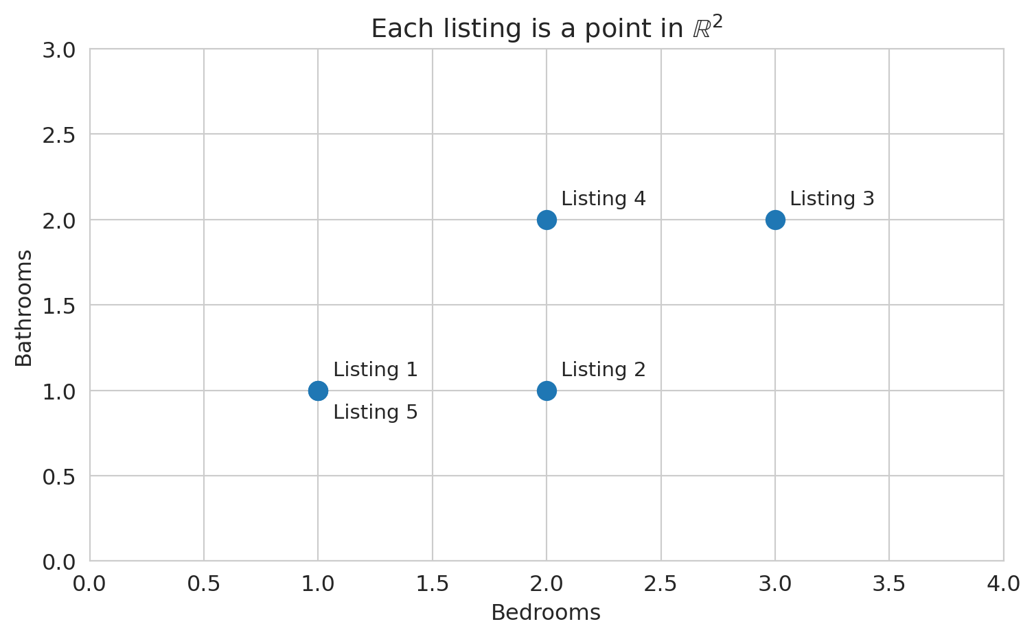
1. **Each row is a vector.** A single Airbnb listing with (bedrooms, bathrooms, price) is a point in $\mathbb{R}^3$. ($\mathbb{R}^3$ just means a list of 3 real numbers — so (2, 1, 150) is a point in $\mathbb{R}^3$.)
2. **Each column is a vector.** The "bedrooms" column across all $n$ listings is a vector in $\mathbb{R}^n$ (one entry per listing).
You'll use both views constantly — and they answer different questions. Let's start with a tiny example to build intuition, then look at real data.
```{python}
# A tiny dataset: 5 Airbnb listings with 2 features
bedrooms  = np.array([1, 2, 3, 2, 1])
bathrooms = np.array([1, 1, 2, 2, 1])

# Each listing is a point in R^2
print(f"Listing 1: bedrooms={bedrooms[0]}, bathrooms={bathrooms[0]}")
print(f"Listing 3: bedrooms={bedrooms[2]}, bathrooms={bathrooms[2]}")
print()
print(f"The 'bedrooms' column is a vector in R^5: {bedrooms}")
print(f"The 'bathrooms' column is a vector in R^5: {bathrooms}")
```
Let's plot the row view: each listing as a point in 2D space, with bedrooms on one axis and bathrooms on the other.
```{python}
# View 1: Each listing as a point in R^2
fig, ax = plt.subplots(figsize=(8, 5))
ax.scatter(bedrooms, bathrooms, s=100, zorder=5)
for i in range(len(bedrooms)):
    offset = (8, 8) if not (i == 4) else (8, -15)
    ax.annotate(f'Listing {i+1}', (bedrooms[i], bathrooms[i]),
                fontsize=11, xytext=offset, textcoords='offset points')
ax.set_xlabel('Bedrooms')
ax.set_ylabel('Bathrooms')
ax.set_title('Each listing is a point in $\\mathbb{R}^2$')
ax.set_xlim(0, 4)
ax.set_ylim(0, 3)
plt.tight_layout()
plt.show()
```
How similar are two listings? One natural measure: multiply corresponding entries and add them up.
```{python}
# How similar are listings 1 and 3?
listing_1 = np.array([bedrooms[0], bathrooms[0]])  # (1, 1)
listing_3 = np.array([bedrooms[2], bathrooms[2]])  # (3, 2)

similarity = listing_1[0] * listing_3[0] + listing_1[1] * listing_3[1]
print(f"Listing 1: {listing_1}")
print(f"Listing 3: {listing_3}")
print(f"Entry-by-entry product sum: {listing_1[0]}*{listing_3[0]} + {listing_1[1]}*{listing_3[1]} = {similarity}")
```
:::{.callout-important}
## Definition: Inner Product (Dot Product)
The **inner product** (or **dot product**) of two vectors $u, v \in \mathbb{R}^n$ is the scalar
$$u \cdot v = u^T v = \sum_{i=1}^n u_i v_i$$
A positive inner product indicates the vectors tend to point in the same direction; a negative value indicates opposite directions; zero indicates perpendicularity.
:::
A word of caution: the raw inner product depends on both direction *and* magnitude. A listing with 10 bedrooms and 10 bathrooms would have a large inner product with almost any other listing, simply from its scale. To isolate directional similarity, divide by the lengths of both vectors — a quantity called **cosine similarity**, which we return to below.
:::{.callout-important}
## Definition: Cosine Similarity
The **cosine similarity** between two vectors $\mathbf{a}$ and $\mathbf{b}$ measures the cosine of the angle between them:
$$\text{cosine similarity} = \frac{\mathbf{a} \cdot \mathbf{b}}{\|\mathbf{a}\| \, \|\mathbf{b}\|}$$
Values range from $-1$ (opposite directions) to $+1$ (same direction). A value of $0$ means the vectors are perpendicular (orthogonal). Cosine similarity measures *direction*, ignoring *magnitude* — two vectors that point the same way have cosine similarity 1 regardless of their lengths.
:::
How large *is* a feature vector? The length generalizes the Pythagorean theorem.
```{python}
# How "big" is each listing's feature vector?
for i, name in [(0, 'Listing 1'), (2, 'Listing 3')]:
    vec = np.array([bedrooms[i], bathrooms[i]])
    length = np.sqrt(vec[0]**2 + vec[1]**2)
    print(f"{name}: {vec}, length = sqrt({vec[0]}^2 + {vec[1]}^2) = {length:.2f}")
```
:::{.callout-important}
## Definition: Norm
The **norm** (or **length**) of a vector $v$ is
$$\|v\| = \sqrt{v \cdot v} = \sqrt{\sum_{i=1}^n v_i^2}$$
The norm measures **magnitude** — how large the vector is. In code: `np.linalg.norm(v)`.
:::
With norms in hand, we can measure how far apart two listings are.
```{python}
# How different are listings 1 and 3?
diff = listing_3 - listing_1
dist = np.linalg.norm(diff)
print(f"Difference vector: {listing_3} - {listing_1} = {diff}")
print(f"Distance = norm of difference = {dist:.2f}")
```
:::{.callout-important}
## Definition: Distance
The **distance** between two vectors $u$ and $v$ is the norm of their difference:
$$d(u, v) = \|u - v\|$$
Smaller distance means more similar. Larger distance means more different.
:::
## Linear functions and linear combinations
:::{.callout-important}
## Definition: Linear Function
A function $f$ is **linear** if it satisfies two properties:
$$f(ax + by) = a\,f(x) + b\,f(y)$$
for all vectors $x, y$ and all scalars $a, b$. Equivalently: scaling the input scales the output, and adding inputs adds outputs.
:::
Familiar examples of linear functions: multiplying by a constant ($f(x) = 3x$), matrix multiplication ($f(x) = Ax$), and the inner product with a fixed vector ($f(x) = w \cdot x$). Non-examples: squaring ($f(x) = x^2$, since $(2x)^2 \neq 2x^2$) and adding a constant ($f(x) = x + 1$, since $f(0) \neq 0$).
Linear models matter precisely for this reason: the prediction $\hat{y} = X\beta$ is a linear function of $\beta$. Changing the weights changes the prediction in a proportional, predictable way — no surprises.
:::{.callout-important}
## Definition: Linear Combination
A **linear combination** of vectors $v_1, v_2$ is any expression $a \cdot v_1 + b \cdot v_2$ where $a, b$ are **scalars** (plain numbers).
:::
A linear model $\hat{y} = \beta_1 \cdot x_1 + \beta_2 \cdot x_2$ says: "the prediction is a linear combination of the feature columns."
Let's see what that looks like. (In code, we write `beta` for the Greek letter $\beta$.)
```{python}
# Two feature vectors (columns of our data matrix)
bedrooms_vec = np.array([1, 2, 3, 2, 1])  # bedrooms column
bathrooms_vec = np.array([1, 1, 2, 2, 1])  # bathrooms column

# A linear combination: 100*bedrooms + 50*bathrooms
beta1, beta2 = 100, 50
prediction = beta1 * bedrooms_vec + beta2 * bathrooms_vec
print(f"Weights: beta1={beta1}, beta2={beta2}")
print(f"bedrooms:    {bedrooms_vec}")
print(f"bathrooms:   {bathrooms_vec}")
print(f"prediction:  {prediction}")
print()
print(f"Listing 1: {beta1}*{bedrooms_vec[0]} + {beta2}*{bathrooms_vec[0]} = ${prediction[0]}")
print(f"Listing 3: {beta1}*{bedrooms_vec[2]} + {beta2}*{bathrooms_vec[2]} = ${prediction[2]}")
```
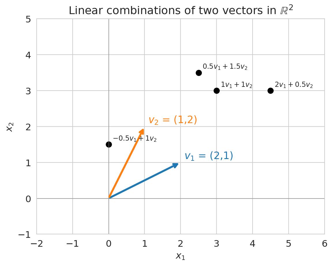
Different weights produce different prediction vectors. The plot below shows several linear combinations of two vectors $v_1$ and $v_2$ in $\mathbb{R}^2$ -- each black dot is one choice of weights.
```{python}
# Visualize linear combinations in 2D
v1 = np.array([2, 1])
v2 = np.array([1, 2])

fig, ax = plt.subplots(figsize=(8, 5))

# Draw the two basis vectors
ax.annotate('', xy=v1, xytext=(0, 0),
            arrowprops=dict(arrowstyle='->', color='C0', lw=2.5))
ax.annotate('', xy=v2, xytext=(0, 0),
            arrowprops=dict(arrowstyle='->', color='C1', lw=2.5))
ax.text(v1[0]+0.1, v1[1]+0.1, '$v_1$ = (2,1)', fontsize=13, color='C0')
ax.text(v2[0]+0.1, v2[1]+0.1, '$v_2$ = (1,2)', fontsize=13, color='C1')

# Show some linear combinations
combos = [(1, 1), (2, 0.5), (0.5, 1.5), (-0.5, 1)]
for a, b in combos:
    lc = a * v1 + b * v2
    ax.plot(*lc, 'ko', ms=7)
    ax.annotate(f'${a} v_1 + {b} v_2$', xy=lc, fontsize=9,
                xytext=(5, 5), textcoords='offset points')

ax.set_xlim(-2, 6)
ax.set_ylim(-1, 5)
ax.set_aspect('equal')
ax.axhline(0, color='gray', lw=0.5)
ax.axvline(0, color='gray', lw=0.5)
ax.set_title('Linear combinations of two vectors in $\\mathbb{R}^2$')
ax.set_xlabel('$x_1$')
ax.set_ylabel('$x_2$')
plt.tight_layout()
plt.show()
```
:::{.callout-tip}
## Think About It
In the plot above, can you reach *every* point in $\mathbb{R}^2$ using linear combinations of $v_1$ and $v_2$? What if $v_1$ and $v_2$ pointed in the same direction?
:::
## Span: the set of all possible predictions
:::{.callout-important}
## Definition: Span
The **span** of a set of vectors is the set of ALL their linear combinations:
$$\text{span}(v_1, v_2) = \{a \cdot v_1 + b \cdot v_2 : a, b \in \mathbb{R}\}$$
:::
In other words, try every possible choice of weights $a$ and $b$. The collection of all the vectors you can make this way is the span.
For a linear model, the span of your feature columns IS the set of all possible predictions. This characterization tells you what your model **can** and **cannot** predict, before you fit anything.
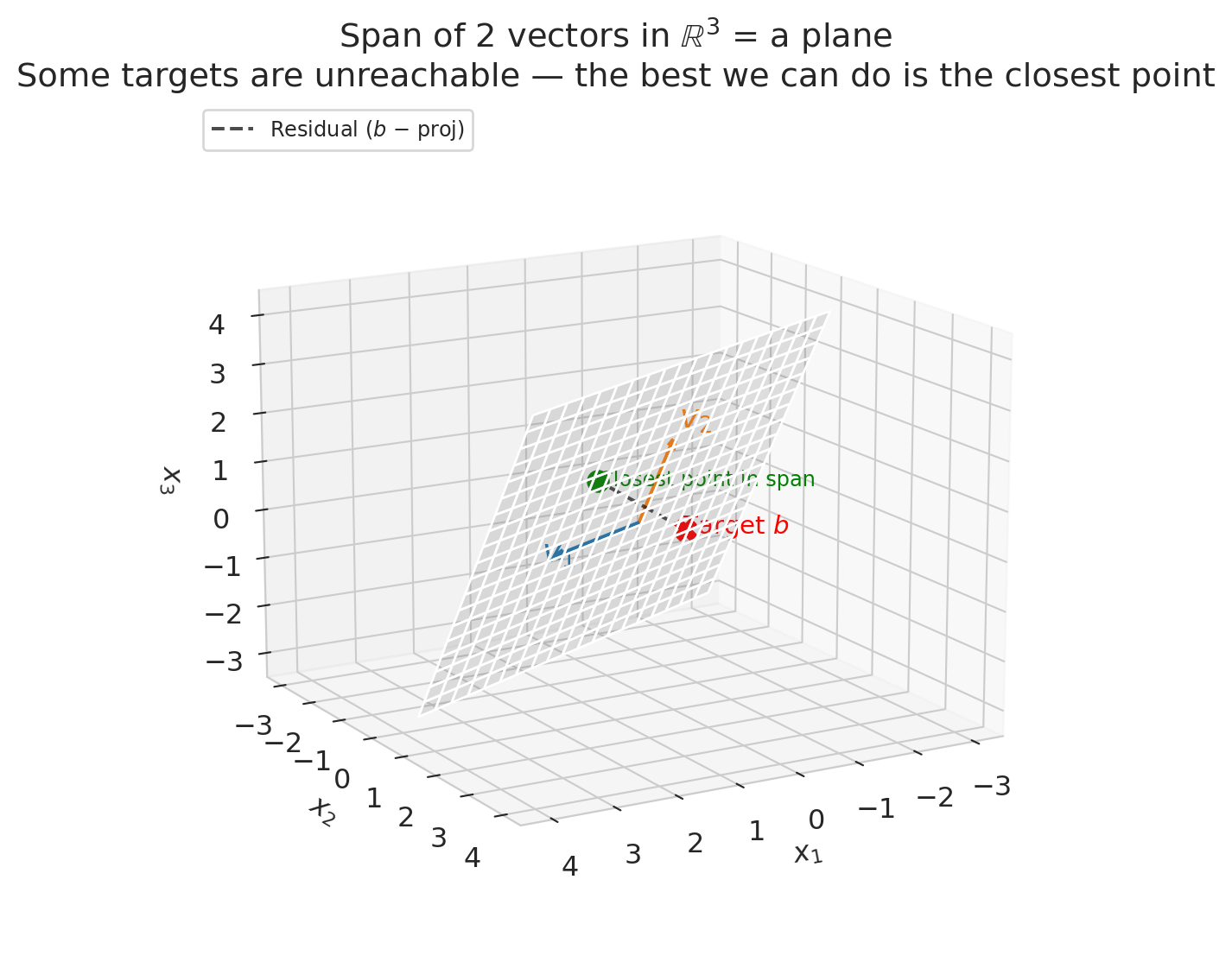
Let's visualize the span of 2 vectors in $\mathbb{R}^3$.
```{python}
from mpl_toolkits.mplot3d import Axes3D

v1_3d = np.array([2, 1, 0])
v2_3d = np.array([0, 1, 2])
target = np.array([1, 3, 1])

# Project target onto span(v1, v2) via least squares
V = np.column_stack([v1_3d, v2_3d])
coeffs = np.linalg.lstsq(V, target, rcond=None)[0]
proj = V @ coeffs

fig = plt.figure(figsize=(8, 6))
ax = fig.add_subplot(111, projection='3d')

# Draw the plane (span) — range covers the projection point
s = np.linspace(-1.5, 2, 20)
t = np.linspace(-1.5, 2, 20)
S, T = np.meshgrid(s, t)
X = S * v1_3d[0] + T * v2_3d[0]
Y = S * v1_3d[1] + T * v2_3d[1]
Z = S * v1_3d[2] + T * v2_3d[2]
ax.plot_surface(X, Y, Z, alpha=0.18, color='gray')

# Draw the two basis vectors
for v, color, label in [(v1_3d, 'C0', '$v_1$'), (v2_3d, 'C1', '$v_2$')]:
    ax.quiver(0, 0, 0, *v, color=color, arrow_length_ratio=0.1, lw=2.5)
    ax.text(*(v * 1.15), label, fontsize=14, color=color)

# Mark the target, its projection, and the residual
ax.scatter(*target, color='red', s=80, zorder=5, marker='X')
ax.text(target[0] + 0.15, target[1] + 0.15, target[2],
        'Target $b$', fontsize=11, color='red')
ax.scatter(*proj, color='green', s=80, zorder=5)
ax.text(proj[0] - 0.3, proj[1] - 0.5, proj[2] - 0.3,
        'Closest point in span', fontsize=9, color='green')

# Dashed line: residual connecting target to its projection
ax.plot([target[0], proj[0]], [target[1], proj[1]], [target[2], proj[2]],
        'k--', lw=1.5, alpha=0.7, label='Residual ($b$ − proj)')

ax.set_xlabel('$x_1$')
ax.set_ylabel('$x_2$')
ax.set_zlabel('$x_3$')
ax.set_title('Span of 2 vectors in $\\mathbb{R}^3$ = a plane\n'
             'Some targets are unreachable — the best we can do is the closest point')
ax.legend(loc='upper left', fontsize=9)
ax.view_init(elev=15, azim=60)
plt.tight_layout()
plt.show()
```
Two vectors in $\mathbb{R}^3$ span a *plane*, not all of 3D space. That means some target values $y$ are impossible to reach exactly — there are targets that no linear combination of your features can produce.
The dashed line in the plot above is the **residual**: the gap between the target and the closest reachable point. In Chapter 5, we'll see that regression finds exactly this closest point — the **projection** of $y$ onto the column space. The residual is what's left over.
## Column space: from features to matrices
In practice, we stack our feature columns side by side into a matrix $X$:
$$X = \begin{bmatrix} | & | \\ x_1 & x_2 \\ | & | \end{bmatrix}$$
:::{.callout-important}
## Definition: Column Space
The **column space** of $X$ is the span of its columns:
$$\text{col}(X) = \text{span}(x_1, x_2) = \{X\beta : \beta \in \mathbb{R}^2\}$$
This set is exactly the collection of all possible predictions $\hat{y} = X\beta$ for a linear model. Different $\beta$ = different predictions, but they all live in the column space.
:::
We build the design matrix $X$ by stacking feature columns side by side using `np.column_stack`. The matrix-vector product `X @ beta` then computes the linear combination for all listings at once.
```{python}
# Build the design matrix from our tiny example
X = np.column_stack([bedrooms_vec, bathrooms_vec])
print("Design matrix X (5 listings x 2 features):")
print(X)
print()
print(f"Column 1 (bedrooms): {X[:, 0]}")
print(f"Column 2 (bathrooms): {X[:, 1]}")
print()

# Any prediction is X @ beta
beta = np.array([100, 50])
y_hat = X @ beta
print(f"With beta = {beta}:")
print(f"Prediction y_hat = X @ beta = {y_hat}")
```
**Key insight:** The column space of $X$ determines what your model can predict. More features (more columns) = larger column space = more possible predictions. But there's a catch...
:::{.callout-warning}
## Linear models can predict impossible values
Nothing stops $X\beta$ from predicting a *negative* price. The column space doesn't know that prices must be positive. Linear models predict what the math allows, not what makes sense. (We'll revisit this limitation when we encounter logistic regression in Chapter 13.)
:::
:::{.callout-tip}
## Think About It
If you have 3 features but one is an exact linear combination of the other two, what is the dimension of the column space? (Hint: it's not 3.)
:::
## Let's look at real data
The toy example let us see the geometry. Now let's check whether these ideas — collinearity, redundant features — actually show up in real Airbnb data.
```{python}
# Load Airbnb data
airbnb = pd.read_csv(f'{DATA_DIR}/airbnb/listings.csv', low_memory=False)

# Clean price column (may contain $ and commas in raw Airbnb data)
airbnb['price_clean'] = (
    airbnb['price'].astype(str).str.replace('[$,]', '', regex=True).astype(float)
)

cols = ['bedrooms', 'bathrooms', 'beds', 'price_clean',
        'accommodates', 'number_of_reviews']
n_before = len(airbnb)
df = airbnb[cols].dropna()
print(f"Dropped {n_before - len(df):,} listings with missing values in {cols}")
df = df[(df['price_clean'] > 0) & (df['price_clean'] <= 500)]
print(f"Working with {len(df):,} listings (after removing NAs and extreme prices)")
df.head(10)
```
Each column of the data frame is now a vector in $\mathbb{R}^n$, where $n$ is the number of listings. Let's inspect the first few entries of each feature column.
```{python}
# Look at the feature columns as vectors
print(f"Each column is a vector in R^{len(df)} (one entry per listing):")
print()
for col in ['bedrooms', 'bathrooms', 'beds']:
    print(f"  {col}: first 8 values = {df[col].values[:8]}")
```
## Let's add another feature
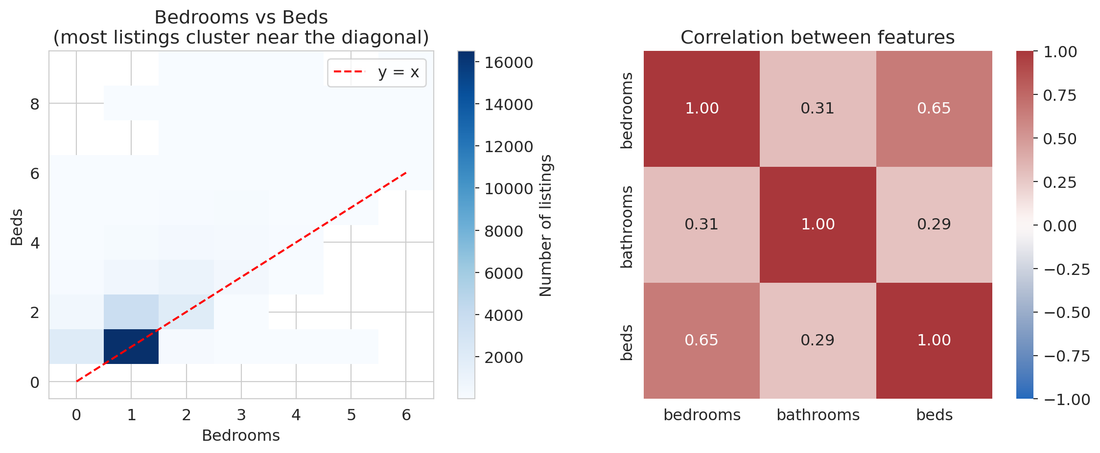
What if two of your features are nearly the same? Let's compare `bedrooms` and `beds`.
```{python}
fig, axes = plt.subplots(1, 2, figsize=(12, 5))

# Left: 2D histogram to show density (many listings stack on same values)
h = axes[0].hist2d(df['bedrooms'], df['beds'], bins=[
    np.arange(-0.5, 7), np.arange(-0.5, 10)],
    cmap='Blues', cmin=1)
plt.colorbar(h[3], ax=axes[0], label='Number of listings')
axes[0].plot([0, 6], [0, 6], 'r--', lw=1.5, label='y = x')
axes[0].set_xlabel('Bedrooms')
axes[0].set_ylabel('Beds')
axes[0].set_title('Bedrooms vs Beds\n(most listings cluster near the diagonal)')
axes[0].legend()

# Right: correlation heatmap
corr = df[['bedrooms', 'bathrooms', 'beds']].corr()
sns.heatmap(corr, annot=True, fmt='.2f', cmap='vlag',
            vmin=-1, vmax=1, ax=axes[1], square=True)
axes[1].set_title('Correlation between features')

plt.tight_layout()
plt.show()

print(f"\nCorrelation between bedrooms and beds: {df['bedrooms'].corr(df['beds']):.3f}")
print(f"Correlation between bedrooms and bathrooms: {df['bedrooms'].corr(df['bathrooms']):.3f}")
```
Bedrooms and beds are positively correlated (r ≈ 0.65). In linear algebra terms, the `beds` vector is nearly a scalar multiple of the `bedrooms` vector:
$$\text{beds} \approx \text{bedrooms}$$
The span barely grows when you add `beds` as a feature. Two vectors pointing in nearly the same direction span almost a **line**, not a **plane**.
The phenomenon is called **multicollinearity**: redundant features that don't expand the column space. High correlation between feature columns corresponds to near-**collinearity** in the column vectors — hence the name.
```{python}
# How parallel are these feature vectors?
# We center first so the angle corresponds to correlation.
bedrooms_centered = df['bedrooms'].values - df['bedrooms'].mean()
beds_centered = df['beds'].values - df['beds'].mean()
bathrooms_centered = df['bathrooms'].values - df['bathrooms'].mean()

cos_beds = np.dot(bedrooms_centered, beds_centered) / (
    np.linalg.norm(bedrooms_centered) * np.linalg.norm(beds_centered))
cos_bath = np.dot(bedrooms_centered, bathrooms_centered) / (
    np.linalg.norm(bedrooms_centered) * np.linalg.norm(bathrooms_centered))

angle_beds = np.degrees(np.arccos(np.clip(cos_beds, -1, 1)))
angle_bath = np.degrees(np.arccos(np.clip(cos_bath, -1, 1)))

print(f"Angle between bedrooms and beds:      {angle_beds:.1f}° (moderate angle)")
print(f"Angle between bedrooms and bathrooms:  {angle_bath:.1f}° (more independent)")
print()
print("When vectors are nearly parallel, adding the second one")
print("barely expands the span. Your model doesn't gain much.")
```
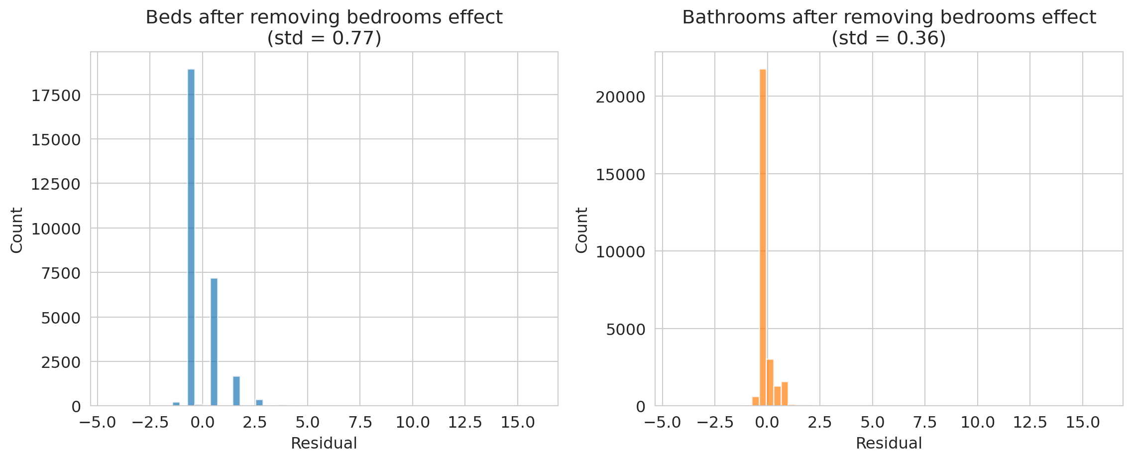
How much independent information does each feature contribute beyond bedrooms? We can project `beds` and `bathrooms` onto the `bedrooms` direction and examine the residual -- the part that bedrooms cannot explain.
```{python}
# What's left after removing the bedrooms component?
# beds ≈ 1.0 * bedrooms + something_else
# The "something_else" is the part that bedrooms can't explain.
# If it's tiny, beds is mostly redundant.

proj_coeff_beds = np.dot(beds_centered, bedrooms_centered) / np.dot(bedrooms_centered, bedrooms_centered)
residual_beds = beds_centered - proj_coeff_beds * bedrooms_centered

proj_coeff_bath = np.dot(bathrooms_centered, bedrooms_centered) / np.dot(bedrooms_centered, bedrooms_centered)
residual_bath = bathrooms_centered - proj_coeff_bath * bedrooms_centered

fig, axes = plt.subplots(1, 2, figsize=(12, 5), sharex=True)

axes[0].hist(residual_beds, bins=50, alpha=0.7, color='C0')
axes[0].set_title(f'Beds after removing bedrooms effect\n(std = {residual_beds.std():.2f})')
axes[0].set_xlabel('Residual')
axes[0].set_ylabel('Count')

axes[1].hist(residual_bath, bins=50, alpha=0.7, color='C1')
axes[1].set_title(f'Bathrooms after removing bedrooms effect\n(std = {residual_bath.std():.2f})')
axes[1].set_xlabel('Residual')
axes[1].set_ylabel('Count')

plt.tight_layout()
plt.show()
print("Bathrooms has much more independent information than beds!")
```
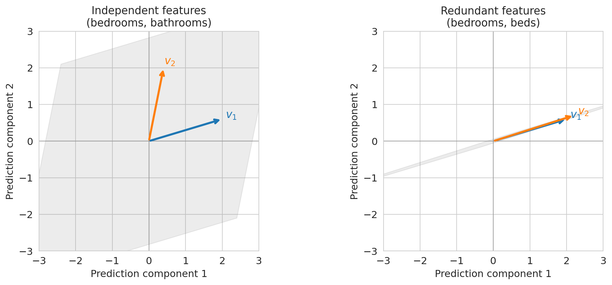
## Visualizing collinearity: 2D span vs near-1D span
Let's make this concrete with a small example. When two feature vectors are **linearly independent** — meaning neither is a scalar multiple of the other — they span a plane. When they're nearly parallel, the "plane" collapses to almost a line.
```{python}
fig, axes = plt.subplots(1, 2, figsize=(12, 5))

panels = [
    (np.array([1, 0.3]), np.array([0.2, 1]),
     'Independent features\n(bedrooms, bathrooms)'),
    (np.array([1, 0.3]), np.array([1.1, 0.35]),
     'Redundant features\n(bedrooms, beds)'),
]

for ax, (va, vb, title) in zip(axes, panels):
    # Shade the span region using a filled polygon
    # The span of two 2D vectors is the region reachable by a*va + b*vb
    corners = []
    for a, b in [(-3, -3), (-3, 3), (3, 3), (3, -3)]:
        corners.append(a * va + b * vb)
    corners = np.array(corners)
    ax.fill(corners[:, 0], corners[:, 1], alpha=0.15, color='gray')

    # Draw the vectors
    for v, color, label in [(va, 'C0', '$v_1$'), (vb, 'C1', '$v_2$')]:
        ax.annotate('', xy=v*2, xytext=(0, 0),
                    arrowprops=dict(arrowstyle='->', color=color, lw=2.5))
        ax.text(*(v*2.1), label, fontsize=13, color=color, fontweight='bold')

    ax.set_xlim(-3, 3)
    ax.set_ylim(-3, 3)
    ax.set_aspect('equal')
    ax.axhline(0, color='gray', lw=0.5)
    ax.axvline(0, color='gray', lw=0.5)
    ax.set_title(title, fontsize=13)
    ax.set_xlabel('Prediction component 1')
    ax.set_ylabel('Prediction component 2')

plt.tight_layout()
plt.show()
```
On the left, two independent features let you reach any point in the plane — you have full 2D freedom. On the right, nearly parallel features only let you move along one direction. **The span collapsed.** Adding the second feature barely helped.
Multicollinearity limits your model: redundant features provide *redundant information*, not new predictive power.
:::{.callout-tip}
## Think About It
If you're an Airbnb host deciding which features to advertise, does it help to list both "bedrooms" AND "beds"? What would you list instead?
:::
## Rank: how many truly independent features do you have?
Vectors are **linearly independent** if none of them can be written as a combination of the others. For example, if $\text{bedrooms} = 0.5 \cdot \text{bathrooms} + 0.3 \cdot \text{beds}$, then bedrooms is **linearly dependent** on the other two — it's redundant.
:::{.callout-important}
## Definition: Rank
The **rank** of a matrix $X$ is the dimension of its column space — equivalently, the number of linearly independent columns.
- If $X$ has 3 columns but rank 2, one column is redundant.
- If rank = number of columns, all features contribute non-redundant information.
:::
Rank is a binary concept: a column is either exactly dependent or it isn't. In code, `np.linalg.matrix_rank(X)` returns the rank. But in practice, *near*-redundancy has a larger effect on model performance, and singular values quantify that effect. Let's check.
```{python}
# Build feature matrices and check rank
features_3 = df[['bedrooms', 'bathrooms', 'beds']].values
features_2 = df[['bedrooms', 'bathrooms']].values

rank_3 = np.linalg.matrix_rank(features_3)
rank_2 = np.linalg.matrix_rank(features_2)

print(f"Matrix with [bedrooms, bathrooms, beds]: shape {features_3.shape}, rank = {rank_3}")
print(f"Matrix with [bedrooms, bathrooms]:        shape {features_2.shape}, rank = {rank_2}")
print()
print(f"All 3 are technically independent (beds != c * bedrooms exactly),")
print(f"so the rank is {rank_3}. But near-collinearity means the 3rd direction")
print(f"adds very little. Singular values reveal how much each direction contributes.")
```
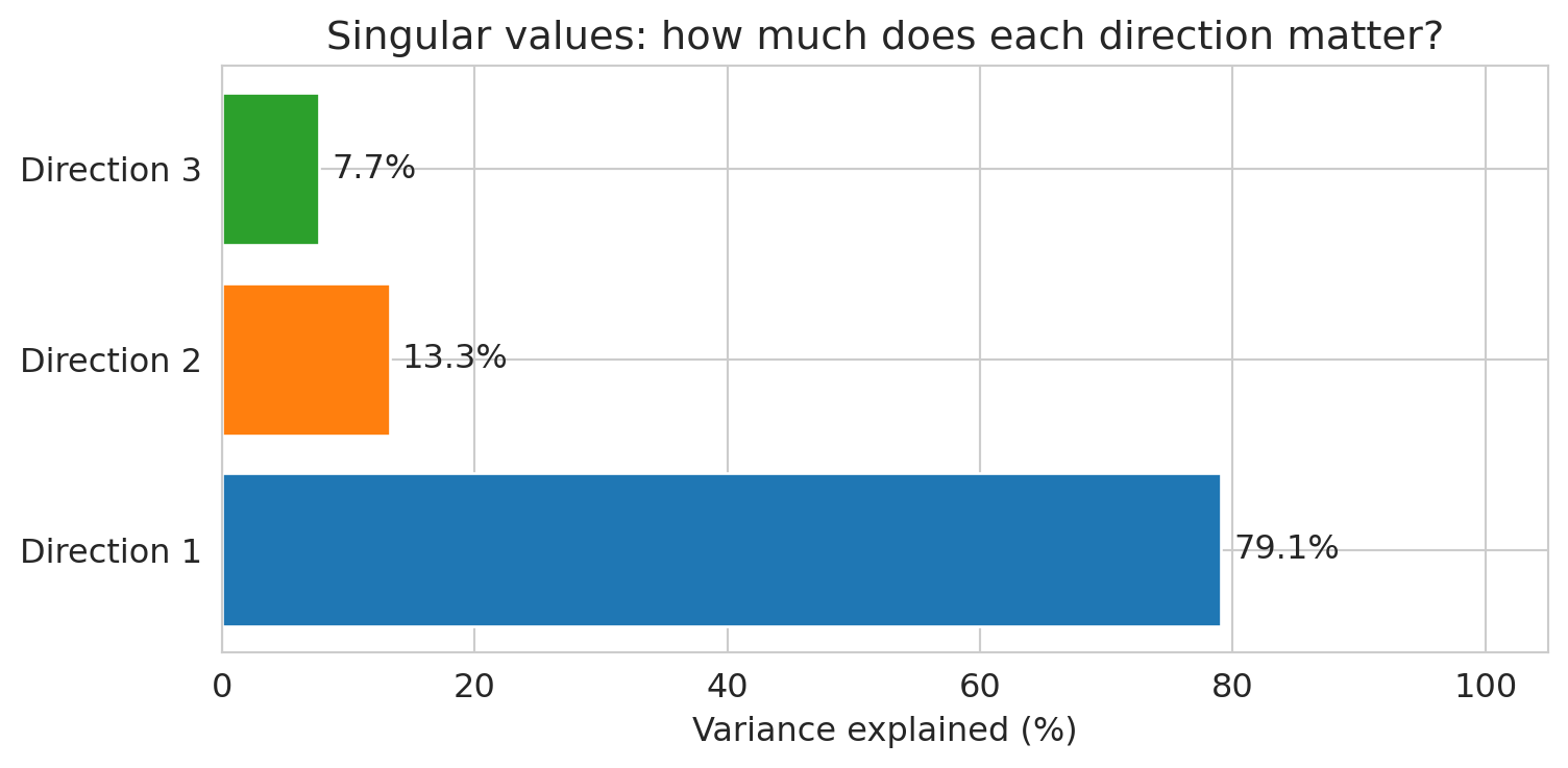
The **singular values** of $X$ (computed by `np.linalg.svd`) quantify how much variance each independent direction captures. We'll study SVD formally in Chapter 14; for now, the bar chart tells the story.
```{python}
# Singular values: how much does each independent direction contribute?
# (We'll return to singular values formally in Chapter 14 on PCA —
#  for now, just look at the bar chart.)
_, singular_values, _ = np.linalg.svd(
    features_3 - features_3.mean(axis=0), full_matrices=False)

# Variance explained is proportional to squared singular values
sv_pct = singular_values**2 / (singular_values**2).sum() * 100

fig, ax = plt.subplots(figsize=(8, 4))
bars = ax.barh(
    [f'Direction {i+1}' for i in range(len(sv_pct))],
    sv_pct, color=['C0', 'C1', 'C2'])
for bar, pct in zip(bars, sv_pct):
    ax.text(bar.get_width() + 1, bar.get_y() + bar.get_height()/2,
            f'{pct:.1f}%', va='center', fontsize=12)
ax.set_xlabel('Variance explained (%)')
ax.set_title('Singular values: how much does each direction matter?')
ax.set_xlim(0, 105)
plt.tight_layout()
plt.show()

print("The 3rd direction contributes very little — beds is mostly redundant with bedrooms.")
```
:::{.callout-tip}
## Think About It
A model with 50 features but rank 3 — what does that tell you about the data? How many features are really doing the work?
:::
## Orthogonality: a preview of regression
One more concept we'll need immediately in Chapter 5.
:::{.callout-important}
## Definition: Orthogonal Vectors
Two vectors $u$ and $v$ are **orthogonal** (perpendicular) if their inner product is zero:
$$u \cdot v = 0$$
For centered data vectors, orthogonality corresponds to zero correlation — the features are **uncorrelated**. Uncorrelated features carry non-redundant information; neither can be predicted from the other by a linear model.
:::
Let's check orthogonality with real feature vectors. Two features with near-zero correlation should have centered vectors that are approximately orthogonal.
```{python}
# Orthogonality computation: are any Airbnb features approximately orthogonal?
# Center the vectors (subtract the mean) so dot product corresponds to correlation
beds_c = df['beds'].values - df['beds'].mean()
reviews_c = df['number_of_reviews'].values - df['number_of_reviews'].mean()
bedrooms_c = df['bedrooms'].values - df['bedrooms'].mean()

# Dot products (unnormalized)
dot_beds_reviews = np.dot(beds_c, reviews_c)
dot_beds_bedrooms = np.dot(beds_c, bedrooms_c)

# Cosine similarity = correlation for centered vectors
cos_beds_reviews = dot_beds_reviews / (np.linalg.norm(beds_c) * np.linalg.norm(reviews_c))
cos_beds_bedrooms = dot_beds_bedrooms / (np.linalg.norm(beds_c) * np.linalg.norm(bedrooms_c))

print(f"beds vs number_of_reviews:")
print(f"  dot product = {dot_beds_reviews:,.0f}")
print(f"  cosine similarity (= correlation) = {cos_beds_reviews:.3f}")
print(f"  angle = {np.degrees(np.arccos(np.clip(cos_beds_reviews, -1, 1))):.1f}°")
print()
print(f"beds vs bedrooms:")
print(f"  dot product = {dot_beds_bedrooms:,.0f}")
print(f"  cosine similarity (= correlation) = {cos_beds_bedrooms:.3f}")
print(f"  angle = {np.degrees(np.arccos(np.clip(cos_beds_bedrooms, -1, 1))):.1f}°")
print()
print("Beds and reviews are nearly orthogonal — they carry independent information.")
print("Beds and bedrooms are far from orthogonal — they carry redundant information.")
```
Why does orthogonality matter? In Chapter 5, we'll see that the residual $e = y - \hat{y}$ from regression is **orthogonal** to the column space of $X$. That orthogonality condition defines the least squares solution and gives us the normal equations.
Orthogonal features (90° apart) expand the column space maximally; parallel features (0°) don't expand it at all.
## What predictions are possible? An answer
The opening of this chapter asked: given your features, what predictions are possible? We now have the tools to answer concretely. The column space of $X$ is the set of all achievable predictions. Any target vector outside the column space cannot be reached exactly — the best a linear model can do is find the closest point inside the column space.
Let's project actual Airbnb prices onto the column space of two feature sets and measure the gap.
```{python}
# Build two design matrices: one with 2 features, one with 4
X_small = df[['bedrooms', 'bathrooms']].values
X_large = df[['bedrooms', 'bathrooms', 'accommodates', 'number_of_reviews']].values
y = df['price_clean'].values

# Project y onto each column space using least squares
beta_small = np.linalg.lstsq(X_small, y, rcond=None)[0]
beta_large = np.linalg.lstsq(X_large, y, rcond=None)[0]

y_hat_small = X_small @ beta_small
y_hat_large = X_large @ beta_large

# Residuals: what the model cannot reach
resid_small = y - y_hat_small
resid_large = y - y_hat_large

print("Projection of actual prices onto the column space:")
print(f"  2 features (bedrooms, bathrooms):")
print(f"    residual norm = {np.linalg.norm(resid_small):,.0f}")
print(f"    avg |residual| = ${np.mean(np.abs(resid_small)):.0f} per listing")
print(f"  4 features (+ accommodates, reviews):")
print(f"    residual norm = {np.linalg.norm(resid_large):,.0f}")
print(f"    avg |residual| = ${np.mean(np.abs(resid_large)):.0f} per listing")
print()
print("More independent features → larger column space → smaller residual.")
```
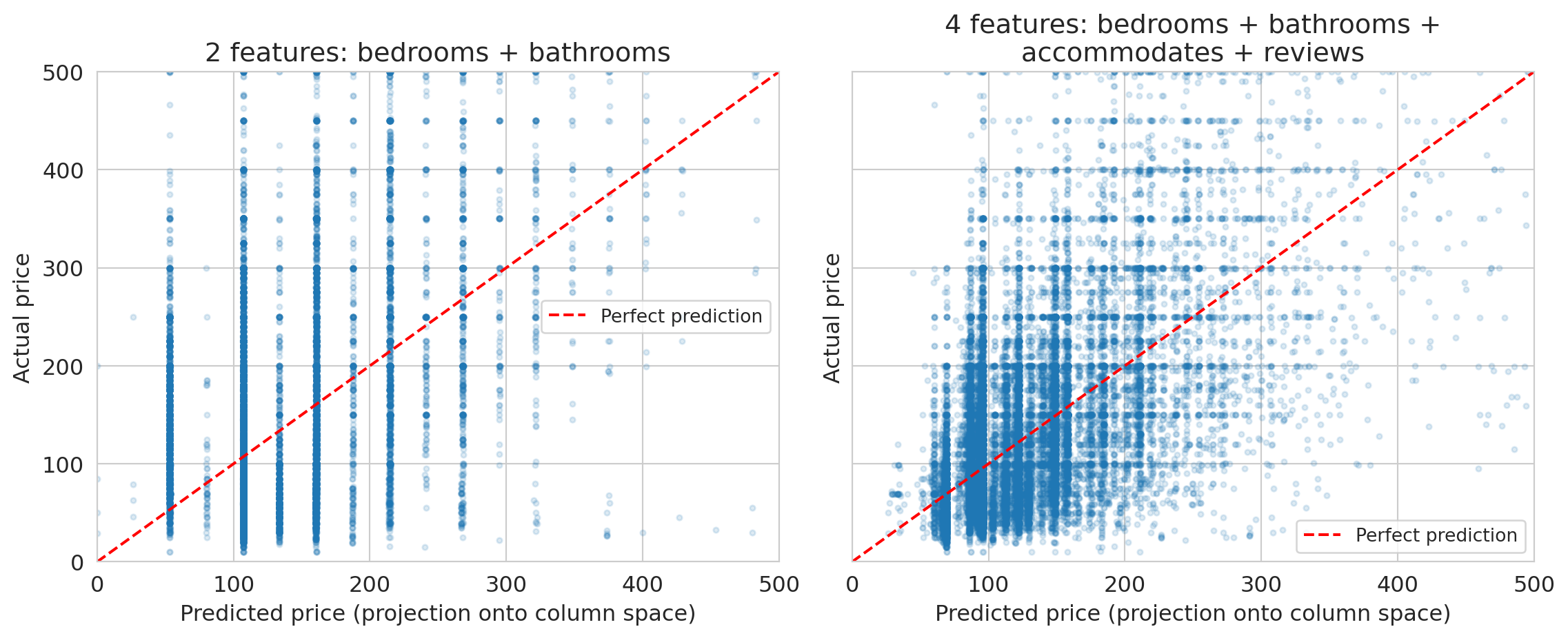
The scatter plots below compare predicted prices (the projection onto the column space, computed by `np.linalg.lstsq`) against actual prices. Points on the red dashed line would be perfect predictions.
```{python}
# Visualize: actual prices vs projected prices
fig, axes = plt.subplots(1, 2, figsize=(12, 5), sharey=True)

for ax, y_hat, label, n_feat in [
    (axes[0], y_hat_small, 'bedrooms + bathrooms', 2),
    (axes[1], y_hat_large, 'bedrooms + bathrooms +\naccommodates + reviews', 4)
]:
    ax.scatter(y_hat, y, alpha=0.15, s=8)
    ax.plot([0, 500], [0, 500], 'r--', lw=1.5, label='Perfect prediction')
    ax.set_xlabel('Predicted price (projection onto column space)')
    ax.set_ylabel('Actual price')
    ax.set_title(f'{n_feat} features: {label}')
    ax.legend(fontsize=10)
    ax.set_xlim(0, 500)
    ax.set_ylim(0, 500)

plt.tight_layout()
plt.show()
```
The gap between the red dashed line and the point cloud is the residual — the part of actual prices that lives outside the column space. A richer column space (more independent features) narrows the gap, but some gap always remains. No linear combination of these features can perfectly reproduce the full complexity of Airbnb pricing.
## Key takeaways
- **Vectors in data**: each feature column is a vector. Each data point is also a vector.
- **Linear combinations**: a linear model predicts $\hat{y} = \beta_1 x_1 + \beta_2 x_2 + \cdots$ — a linear combination of feature columns.
- **Span and column space**: the set of all possible predictions IS the column space of $X$. It tells you what your model *can* and *cannot* do.
- **Collinearity**: if two features are nearly parallel (like `bedrooms` and `beds`), the column space doesn't grow. You get redundancy, not new predictive power.
- **Rank**: the rank of $X$ tells you how many *truly independent* features you have. Singular values tell you how much each one contributes.
Linear algebra tells you what your model CAN and CANNOT do, **before you fit anything.**
In Chapter 6, we'll see that choosing the right features — polynomial terms, interactions, category indicators — lets linear models capture nonlinear patterns.
## Further reading
Want to build more intuition? The [3Blue1Brown "Essence of Linear Algebra"](https://www.3blue1brown.com/topics/linear-algebra) series is excellent and requires no prerequisites — watch at least episodes 1–4.
For a deeper formal treatment: **VMLS** (Boyd & Vandenberghe), Chapters 1 (Vectors) and 5 (Linear independence).
Next chapter: we'll use these ideas to understand *why* the linear regression formula works. Specifically, regression finds the **projection** of $y$ onto the column space — the closest reachable prediction to the actual target.
## Study guide
### Key ideas
- **Vector**: an ordered list of numbers. Each feature column and each data row is a vector.
- **Linear function**: $f$ is linear if $f(ax + by) = af(x) + bf(y)$. Linear models are linear in the weights $\beta$.
- **Inner product (dot product)**: $u \cdot v = \sum u_i v_i$ — measures similarity between vectors (but depends on magnitude; use cosine similarity to isolate direction).
- **Cosine similarity**: $\cos\theta = \frac{u \cdot v}{\|u\|\|v\|}$ — directional similarity, independent of magnitude. Equals correlation for centered vectors.
- **Norm**: $\|v\| = \sqrt{v \cdot v}$ — the length/magnitude of a vector.
- **Distance**: $d(u,v) = \|u - v\|$ — measures dissimilarity between vectors.
- **Orthogonal**: vectors with zero inner product; for centered data, orthogonality means zero correlation (uncorrelated).
- **Linear combination**: $a \cdot v_1 + b \cdot v_2$ — a weighted sum of vectors. A **scalar** is a single number used as a weight.
- **Span**: the set of all linear combinations of a set of vectors.
- **Column space**: the span of the columns of a matrix $X$ — equivalently, the set of all possible predictions $X\beta$.
- **Linearly independent**: vectors are linearly independent if none can be written as a combination of the others.
- **Collinearity / multicollinearity**: when feature vectors are nearly parallel, so one is approximately a scalar multiple of another.
- **Rank**: the number of linearly independent columns in a matrix.
- A linear model's predictions live in the column space of $X$.
- Nearly parallel features don't expand the column space — you get redundancy, not predictive power.
- Rank tells you how many truly independent features you have; singular values tell you how much each contributes.
- When the target $y$ isn't in the column space, the best prediction is the closest point in the span (the projection — Chapter 5).
### Computational tools
- `np.dot(u, v)` or `u @ v` — inner product (dot product)
- `np.linalg.norm(v)` — Euclidean norm (length) of a vector
- `np.column_stack([a, b])` — build a design matrix from column vectors
- `np.linalg.matrix_rank(X)` — rank of a matrix
- `np.linalg.svd(X)` — singular value decomposition (more in Chapter 14)
- `df.corr()` — correlation matrix (related: high correlation ↔ near-collinearity)
### For the quiz
- Be able to determine whether a vector is in the span of given vectors.
- Know what happens to the column space when you add a redundant feature.
- Understand the connection between rank and the number of independent features.
- Know what collinearity means and why it's a problem for prediction.