Lecture 16: When validation isn’t enough

MSE 125 — Applied Statistics

Madeleine Udell

Wednesday, May 20, 2026

logistics

• HW 4 (HMDA mortgage challenge) due Mon May 25
• project final: keep building; group work reminder
• today: validation failures in deployment

START RECORDING.

HW 4 is the HMDA Kaggle challenge, due Monday. Today is the capstone of the “trust models” act: everything we’ve built — train/test, cross-validation — rests on assumptions, and today is about what happens when those assumptions break in deployment.

you shipped a model that passed validation

• it cleared every train/test check
• in deployment it quietly falls apart

what did the random split miss?

The recurring nightmare of anyone who deploys models. You did everything right — held out a test set, cross-validated, reported an honest number. The model still fails in the wild. This lecture names four reasons why, mildest to deepest. Don’t reveal them yet; let the question sit.

agenda

• temporal leakage
• distribution shift
• feedback loops
• Goodhart’s law
• what to do

Five blocks. The first three are validation-technique failures — fixable with the right split or stress test. The last two are deeper: the model is part of the world it predicts.

validation rested on three assumptions

from Chapter 6:

• rows are exchangeable: order doesn’t matter
• deployment matches training
• predictions don’t affect outcomes

this lecture: when each one breaks

Chapter 6 built validation on these three. Every one can fail. The order today is mildest to deepest — exchangeability first, the predictions-affect-outcomes assumption last.

four ways the assumptions break

failure mode	what happens	fix
temporal leakage	random split leaks information about the test set	train past, test future
distribution shift	deployment regime never seen	monitor accuracy after deployment
feedback loops	prediction changes the outcome	randomized holdout
Goodhart’s law	metric becomes a target	audit proxy vs. goal

The spine of the whole lecture. Reveal the rows one at a time if you like. The “fix” column gets less and less satisfying as you go down — by the time you reach Goodhart, no split saves you.

temporal leakage

the data: US monthly retail sales

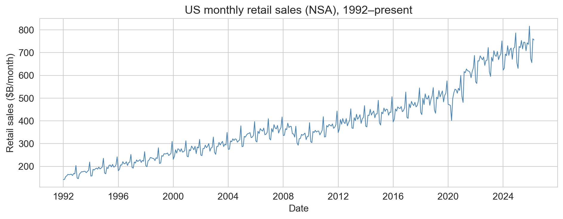
US Census / FRED series RSAFSNA, not seasonally adjusted

• long-run trend: sales grow with population, prices
• annual cycle: sharp December spike, January trough
• short-range autocorrelation: this month ≈ last month

Our running dataset for the time-series half. Not seasonally adjusted, so all three kinds of structure are on display. Each one matters: each suggests a different model, and each interacts differently with how we split.

non-stationarity

non-stationary series

a time series whose mean or variance changes over time

here: retail sales climbs year after year, and the December spike grows with it

non-stationarity is what makes time-series validation different from the i.i.d. (independent, identically distributed) world of Chapter 6

The mean isn’t fixed — it trends up. The seasonal swing widens. This is the structural fact that breaks the exchangeability assumption.

scoring a forecast: MAE

mean absolute error (MAE)

\text{MAE} = \frac{1}{n}\sum_{i=1}^{n}\left| y_i - \hat{y}_i \right|

average size of the forecast error, in the units of the target (here, dollars). lower is better

We need a number to score forecasts and a baseline to beat. MAE is the average miss in dollars. Robust to the occasional huge error in a way RMSE isn’t.

the bar to clear: naive baseline

• strongly seasonal series → same month last year \hat{y}_t = y_{t-12}
• fits no parameters, uses no features

Naive (same month last year) MAE, full series: $20.3B

any model that can’t beat this isn’t earning its complexity

For a non-seasonal series the analogue is the persistence forecast: next step equals this step. The naive baseline is the honest yardstick — beat it or justify the extra machinery.

same data, two ways to split

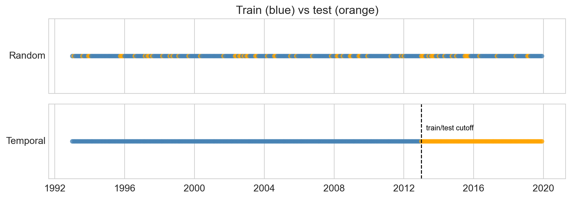
• random: shuffle all months, hold out 20%
• temporal: train early years, test later ones

The model is fixed; only the evaluation changes. The temporal split mimics deployment: train on the past, predict the future. The random split does not — and on a time series, that difference is everything.

data leakage

data leakage (temporal)

information unavailable at prediction time contaminates training, producing optimistically biased scores

here: a random split puts a 2010 test month’s immediate neighbors (the months just before and after) into the training set

Leakage is the general failure; the random-split-on-time-series is the specific instance. The model gets to peek at observations it would never have at deployment.

three forecasts, three kinds of structure

lag features

predictors built from the series’ own past values

• recent lags: last month, last quarter’s average → momentum
• linear trend: a straight line through time → long-run growth
• seasonal: sine/cosine of the month + the year-ago value → annual cycle

why sine/cosine, not a dummy per month? 12 monthly dummies cost 11 extra parameters and overfit a short history. two Fourier features, sin and cos, impose one smooth annual shape

Each model is built from lag features — past values of the series used as predictors for the present. Each leans on a different kind of structure. Name the term “lag features” here; it’s the quiz vocabulary and the operational vocabulary (“lag12”, “year-ago anchor”) all comes back to it.

The seasonal bullet hides a feature-engineering choice worth naming. The obvious way to encode “which month is it?” is twelve one-hot dummies — but that spends eleven free parameters, and with only a few dozen Januaries in the training window each monthly effect is estimated from little data and chases noise. The sine/cosine pair are Fourier features: they impose a single smooth wave that repeats every 12 months, capturing the annual cycle with two parameters instead of eleven. We use them here for that parsimony; with abundant data and a genuinely irregular month-to-month pattern, dummies can win.

predict before you see the answer

three forecasting models: recent lags, linear trend, seasonal

all score R² > 0.9 on a random split.

which still perform well when we train on the past and test on the future?

DISCUSSION: Predict-then-reveal (3 min). Hands or quick poll: which of the three survive a temporal split? Take a vote before the reveal.

Recent lags = last month + last quarter’s average. Linear trend = a straight line through time. Seasonal = sine/cosine of the month + same-month-last-year.

If stuck: “which model leans hardest on its near neighbors in time?”

Key insight: the two that depend on nearby points (momentum, a local line) collapse; only the year-ago anchor survives. The reveal table is next.

the reveal: random hides what temporal exposes

Model            random R²  temporal R²  temporal MAE
-----------------------------------------------------
Recent lags          0.907        0.378        $27.2B
Linear trend         0.933        0.446        $26.1B
Seasonal             0.975        0.936         $9.3B
Naive baseline           —        0.847        $15.9B

• random split: all three excellent
• temporal split: recent-lags & trend fall below the naive baseline
• same models, same data: only the split changed

R² closer to 1 is better; MAE in $B, lower is better

This is the centerpiece. Read down the columns. The random-split column is what a careless evaluation reports; the temporal column is what deployment delivers. The verdict swings from “all excellent” to “two lose to a forecast that fits no parameters.”

why does only the seasonal model validate well?

• random test month sits between its neighbors: easy to interpolate
• temporal test month: training data ends years earlier
  • trend extrapolates a line → falls behind as growth compounds
  • recent lags: only short-range structure to lean on
  • seasonal: carries the year-ago value + a stable annual shape

leakage bites the models whose accuracy needs neighbors nearby in time

The random split didn’t make those models bad — they were always going to struggle out of sample. It just hid it. A random number answers “how well does this interpolate inside data it has seen?” The temporal number answers “how well will it forecast?” Only the second is the job.

walk-forward validation

walk-forward validation

repeat the temporal split at many cut points: train on an expanding window, test the next period, step forward

Fold 1: [===== TRAIN =====][TEST]
Fold 2: [======= TRAIN =======][TEST]
Fold 3: [========= TRAIN =========][TEST]

• expanding window keeps all history; sliding uses a fixed width
• called backtesting in finance

One temporal split gives one number from one cut point. Walk-forward gives many, and shows when a model breaks, not just an average. Sliding windows help when old data comes from a different regime.

when does the model break?

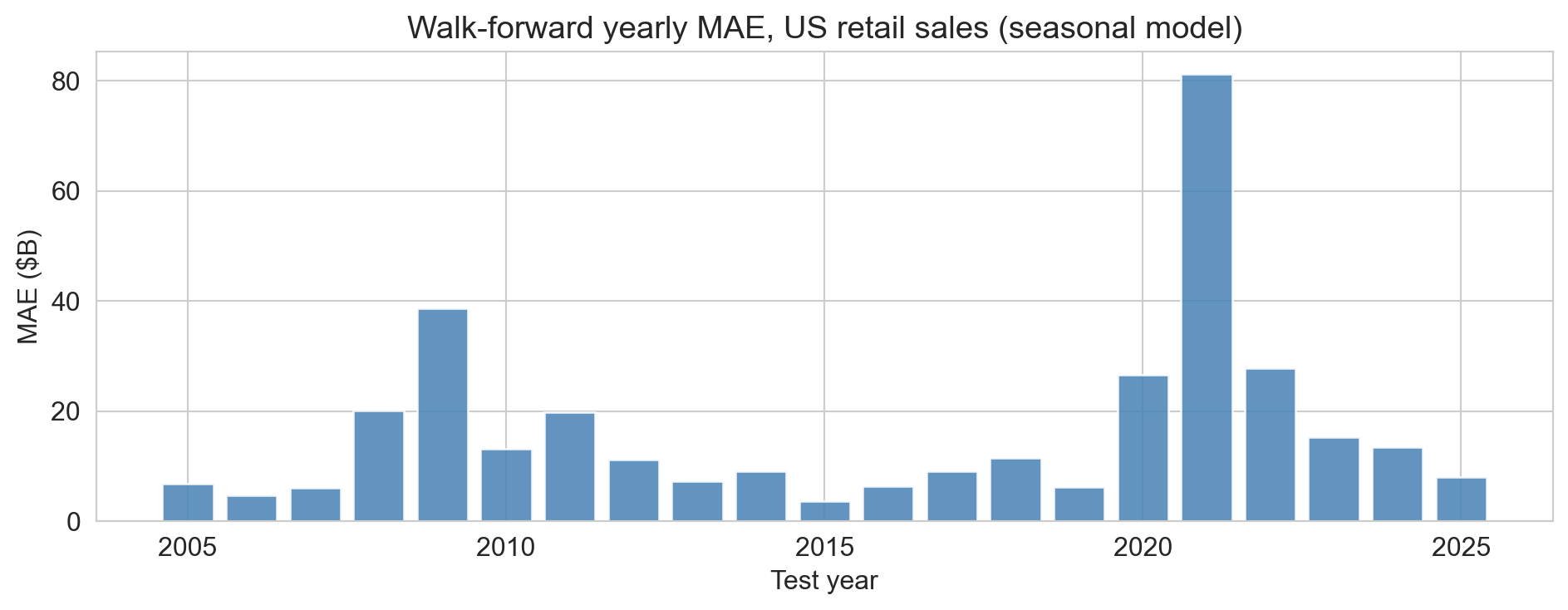
• low error through the calm years
• spikes: 2008–09 crisis, far larger 2020 pandemic
• a single average MAE would bury these regime changes

The spikes are regime changes — the distribution shift of Part 3. Walk-forward surfaces when the model fails. For ordinary years the seasonal model is serviceable, but it imposes one fixed annual shape across three decades. Part 2 builds a model that adapts.

split by the right axis

• a churn model predicts which customers will cancel
• data: one row per customer per month (each customer recurs many times)

split at random by row? or some other way, and why?

DISCUSSION: Think-pair-share (4 min). Think and jot; pair and compare; debrief.

If stuck: “if the same customer is in both train and test, what has the model effectively seen?”

Key insight: split by customer, not by row — otherwise the model sees a customer’s other months at training time, the same leakage as the time series. The general lesson: ask what generalization axis you care about, and split along it.

match the model to the structure

decompose: trend × seasonal × residual

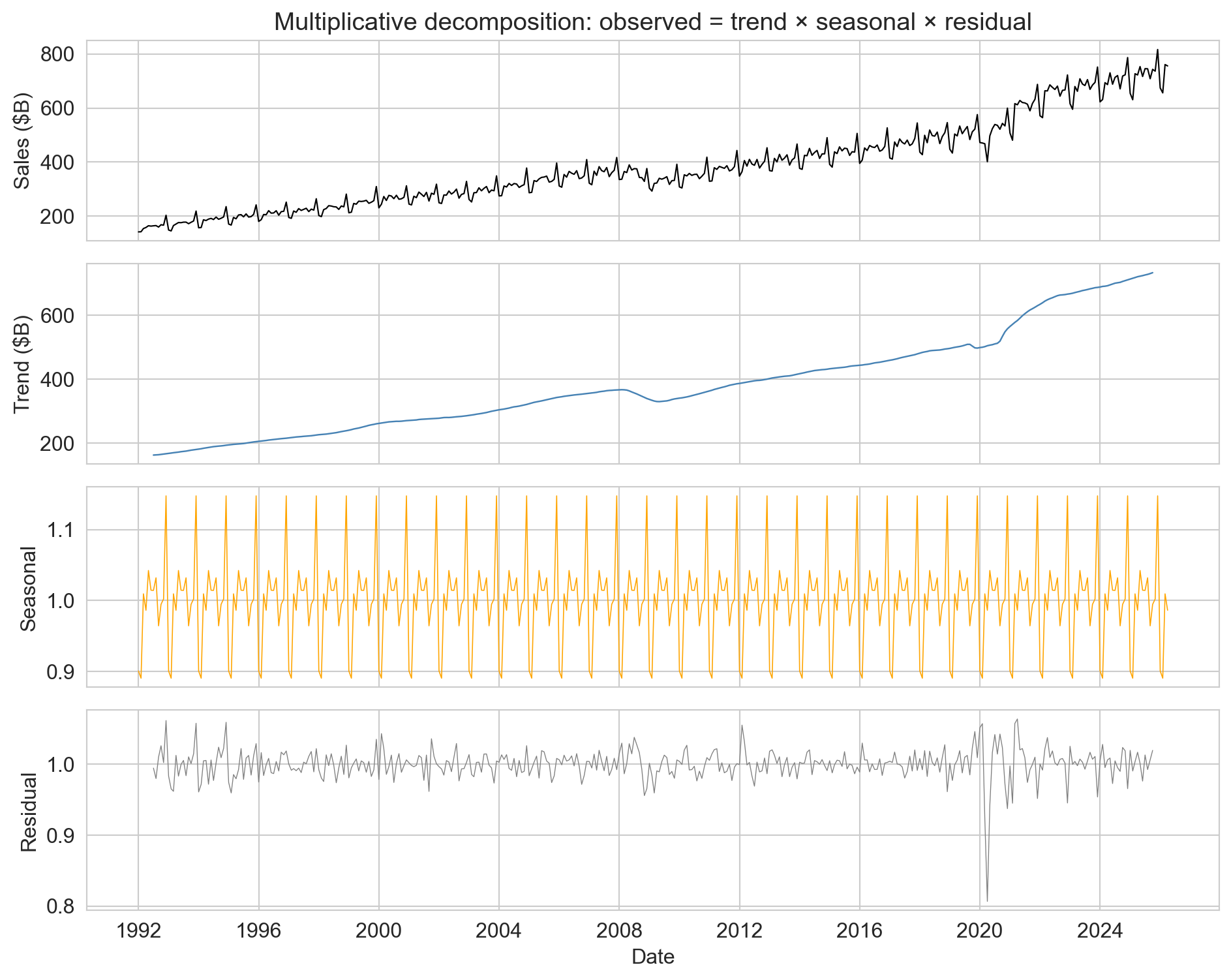
• multiplicative: December is the same percentage above trend each year
• seasonal multiplier: Dec 1.147 (+15% above trend), Feb 0.891
• residual small except the COVID crater

Classical decomposition makes the structure explicit. Retail is multiplicative — the December spike is +15% on trend, not a fixed dollar amount. Outside crises the residual is tiny: trend plus seasonality already captures most of the variation.

Holt-Winters: let the structure adapt

• tracks level, trend, seasonal: each re-estimated as data arrives
• three smoothing parameters \alpha, \beta, \gamma \in [0,1]: how fast each adapts (near 1 chases recent data, near 0 barely moves)
• state only ever looks backward → extends naturally into the future

alpha (level)    = 0.502
beta  (trend)    = 0.000
gamma (seasonal) = 0.204

\beta \approx 0: the growth rate barely changes year to year

Decomposition forced one fixed trend and one seasonal shape. Holt-Winters lets all three drift. Its backward-only construction is the modeling counterpart of walk-forward evaluation. The fitted beta near zero confirms the intuition: the slope is stable, so the trend update barely moves.

demo: forecasting retail sales

switch to the notebook

• naive vs linear regression vs Holt-Winters
• 24-month forecast (2018–19), trained through 2017

colab: lec16-feedback-loops.ipynb

The model comparison is exploratory — fit three models, forecast two years, score them. Run it live in the notebook rather than walking through code on slides.

the forecast, and the verdict

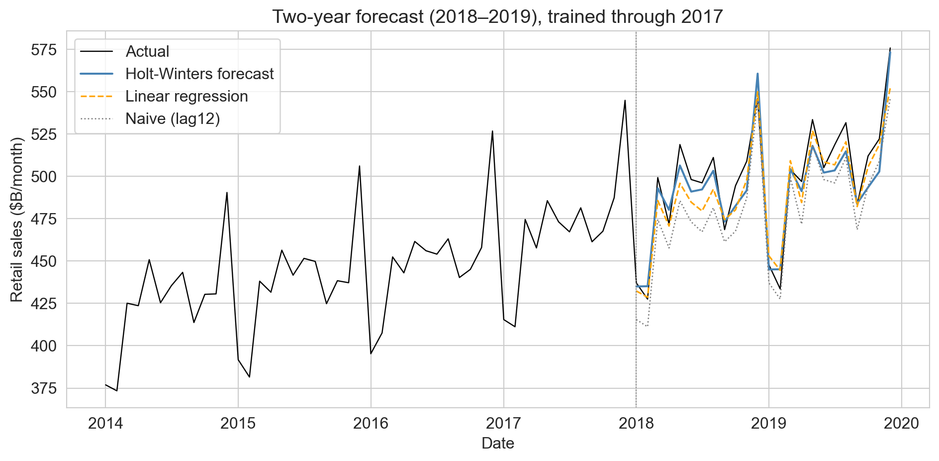
Model                                R²       MAE
Naive (lag12)                     0.672    $18.2B
Linear regression (lag12+trend)   0.894     $9.5B
Holt-Winters                      0.907     $9.0B

Holt-Winters wins by tracking the December multiplier. but a better model still doesn’t fix validation: COVID breaks any fit trained through 2019

Both models clear the naive bar. Matching the model to the structure — adaptive trend, multiplicative seasonality — is the right starting point for sales, energy, traffic, electricity load. But switching models doesn’t fix validation: the COVID shock still breaks any fit trained through 2019.

distribution shift

the data: California daily AQI

retail had clean repeating structure. now a series with almost none

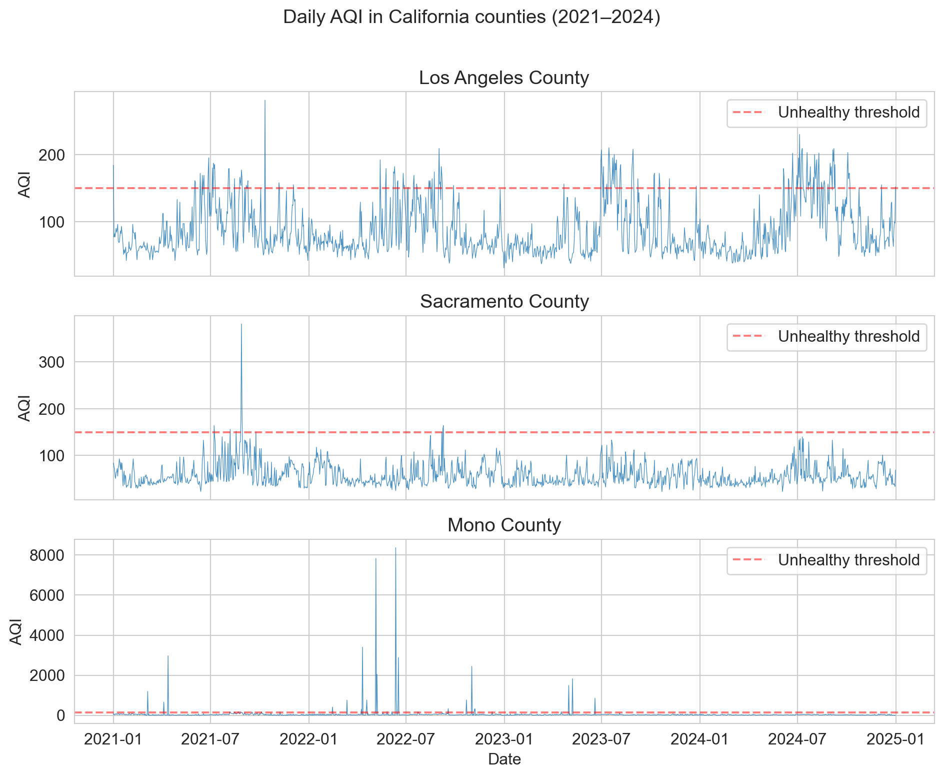
• LA, Sacramento: seasonal wildfire spikes on baseline pollution
• Mono County: dust storms push AQI above 8,000
• AQI: 0 clean → 150 unhealthy → 500 hazardous

EPA daily Air Quality Index. Almost no long-run trend — just short-range noise punctuated by smoke and dust that push the series into territory no training set contained. The same lag-feature toolkit applies; the lesson is what happens at the tails.

predict the failure

train a linear model on yesterday’s AQI, using only normal days (AQI < 300).

a dust storm hits: actual AQI = 8,000.

does it get close, or badly miss? roughly what does it predict?

DISCUSSION: Predict-then-reveal (2 min). Quick poll on the predicted value — will it get close, or badly miss?

If stuck: “what does the model know about days like this? how many were in training?”

Key insight: it predicts near the training mean (~30) and misses by thousands. The reveal is next. The point: it didn’t refuse to extrapolate — the signal it needed was never in the training data.

the model flatlines

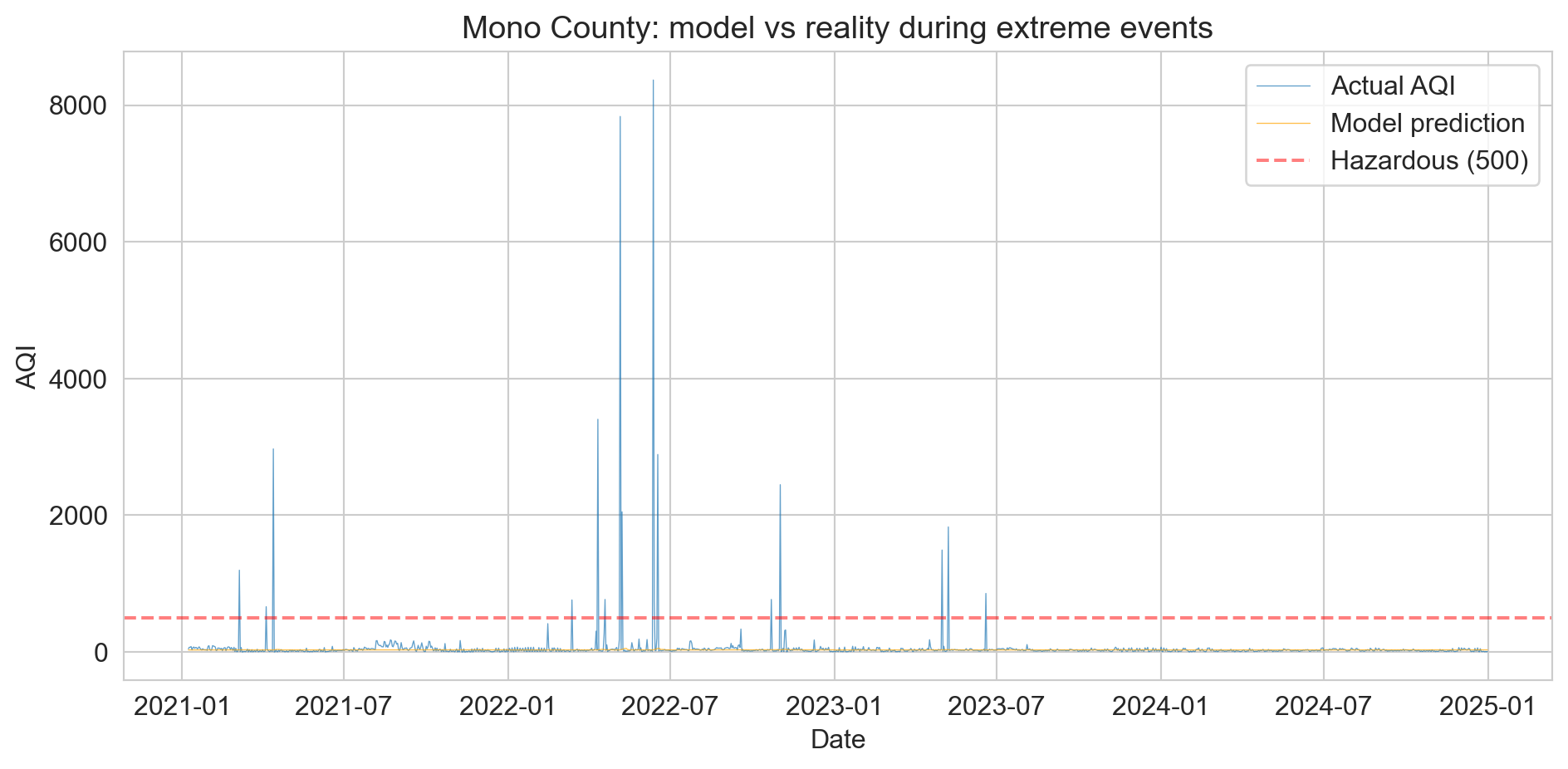
selected extreme days
Actual AQI    Predicted    Error
      7835           30     7805
      3404           30     3374
      1196           29     1167

coefficient on yesterday’s AQI ≈ −0.0004

Why does it fail even when yesterday was extreme? Inside the training range (AQI < 300), day-to-day changes are dominated by noise, so OLS learns lag1 carries little signal and settles near the mean. Plug in 8,000 and the prediction barely moves. The signal it needed wasn’t there to learn.

distribution shift

distribution shift

future data comes from a different regime than the training data: a qualitative change the training set never captured

the events that matter most (wildfires, pandemics, crashes) are the ones your model has never seen

no cross-validation fixes this: it holds out points that look like training data

“prediction is very difficult, especially about the future” (attr. Bohr)

A severe form of non-stationarity. Cross-validation guards against in-distribution noise, not against a future that breaks the pattern. Chapter 17 returns to this: AutoML tools default to standard CV and don’t know your data is temporal.

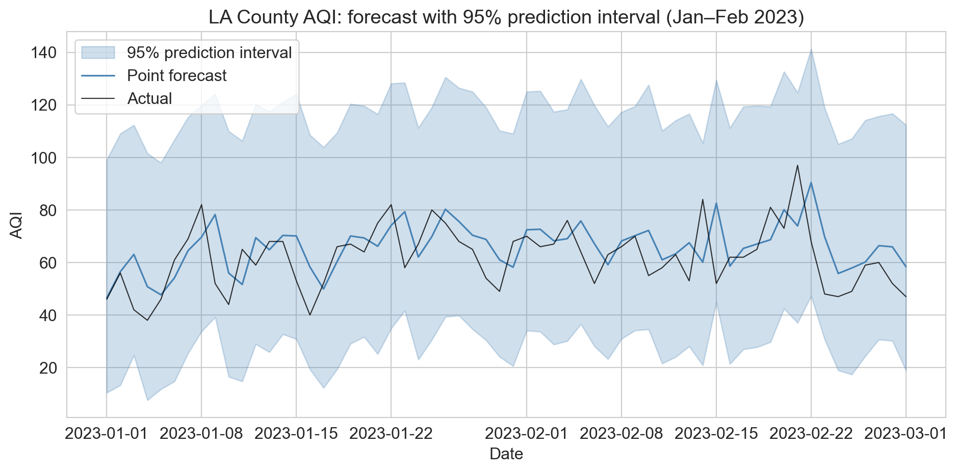
report a range, not a point

• bootstrap from Chapter 8: resample training residuals, add to each forecast
• works for any model: 95% interval here, coverage 93.7%, width 89.5 AQI
• widens for ordinary noise, but blind to regimes never seen (Mono blew past it)

A point forecast hides what a decision-maker needs: should the county issue an advisory? That depends on whether “62” means “55–70” or “could be 200.” The interval widens for ordinary noise — but it’s blind to regimes the training data never held. A forecast without a range isn’t a complete forecast.

when predictions change the world

predictive policing

Photo: Mr. Satterly / Wikimedia Commons, CC0

• model flags neighborhood as high-crime
• police patrol it harder
• more patrols → more arrests
• model retrains, “confirms” itself

. . .

the model creates the data that justifies it

The prediction is self-fulfilling. This isn’t confounding, where the association already exists and we misread it — here the model causes the association. Even a clean temporal split won’t save you, because the model is part of the world it predicts.

a causal arrow runs backward

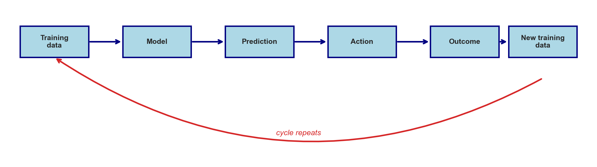
prediction → action → outcome → new training data → repeat

“Correlation is not causation” isn’t the whole story — sometimes the model is the cause. When predictions change the data-generating environment, the test set no longer represents the deployed world, and validation breaks down.

feedback loops are everywhere

• credit scoring: low score → denied loans → no history → score stays low
• recommendations: extreme content → engagement → more extreme
• sepsis alerts: treat flagged patients earlier → fewer cases → model looks worse
• betting markets: the line already encodes your signal

The sepsis case is the subtle one: post-deployment the model looks worse not because it degraded, but because the outcome it predicted stopped happening. Retraining on post-deployment data only makes it circular. The betting market is the feedback loop — sharp money has already moved the line to your signal.

ask before you deploy

will the predictions change the data distribution?

safe	feedback loop
weather forecasts	credit scores
particle-physics models	sepsis alerts

forecasters don’t change the weather; credit scores change who gets loans

A clean test. If predictions feed back into the environment, no held-out set tells you how the model will behave. You need a randomized holdout or an A/B test.

Weapons of Math Destruction

Photo: GRuban / Wikimedia Commons, CC BY-SA 4.0

three traits together make a WMD:

1. outcome not easily measurable
2. negative consequences for individuals
3. self-fulfilling feedback loop

Cathy O’Neil, Weapons of Math Destruction (2016)

O’Neil’s framework. The three traits compound: an unmeasurable outcome means you can’t compute a clean test error, harm means the stakes are real, and the loop means the model entrenches its own bias. All three together is what turns an ordinary model into a weapon.

WMD or not?

• college rankings: high rank attracts students, faculty, donors → raises quality → validates the rank
• parole risk: longer prison can raise reoffense odds (lost job, networks) → confirms the prediction
• weather, particle physics: not WMDs

Both top examples hit all three traits. Weather and particle physics fail trait 3 — the prediction doesn’t change the thing measured. Use these to calibrate the definition before the discussion.

is this a Weapon of Math Destruction?

a model predicts which students will fail a course; the university uses it to assign tutoring.

check the three traits:

1. is the outcome (failing) measurable?
2. could the prediction harm students?
3. does it create a loop?

DISCUSSION: Design challenge (6 min). Small groups: walk the three traits, then propose one design change.

Traits to check: is the outcome (failing) measurable? Could the prediction harm students through stigma or self-fulfilling expectations? Does it create a loop?

Key insight: the use determines the verdict. Tutoring is a virtuous intervention that breaks the loop — it changes the outcome in the helpful direction and the harm is low. Flag-and-punish would be a WMD. Same prediction, opposite design.

“when a measure becomes a target,
it ceases to be a good measure”

Goodhart 1975; popularized by Strathern

Goodhart’s law is game-theoretic

• attach consequences to a metric M
• the agents being measured respond
• those best at gaming M benefit disproportionately

three ingredients:

1. a proxy M for the goal G we care about
2. consequences tied to M (money, status, survival)
3. agents who can move M, and differ in how well

Not just overfitting. Before the metric carries stakes, M and G may be tightly linked. After, M reflects a mix of G and skill-at-gaming-M. The data M collects afterward isn’t the data it was calibrated on.

emissions testing

• VW software detected the EPA lab cycle
• full emissions controls only during the test
• on the road: NOx up to ~40× the legal limit

. . .

optimized the test exactly. real-world emissions moved the opposite way

Photo: Mario R. Duran Ortiz / Wikimedia Commons, CC BY-SA 3.0; EPA Notice of Violation 2015

The cleanest Goodhart case. The proxy was lab-cycle emissions; the goal was clean air. VW optimized the proxy perfectly and the goal got worse. Surfaced through on-road testing by West Virginia University, commissioned by the ICCT.

school accountability tests

when evaluations hinge on scores:

• Chicago: answer-altering in ≥ 4–5% of classrooms
• Florida: weak students reclassified as test-exempt

. . .

the score rises without learning rising

Photo: dcJohn / Wikimedia Commons, CC BY 2.0; Jacob & Levitt 2003, Figlio & Getzler 2002

Two distinct gaming strategies: outright cheating, and changing who gets counted. Both move the measured score without moving the underlying goal. The agents are teachers and administrators responding to stakes.

the same shape, everywhere

• hospital readmissions: hold patients in “observation,” divert to the ED
• citations & h-index: coercive citation, citation cartels
• p-hacking: try analyses until one clears p < 0.05

attach stakes → behavior changes → the numbers stop meaning what they did

Wadhera et al. 2018; Wilhite & Fong 2012; Fister et al. 2016; Simmons et al. 2011

Readmission penalties: hospitals lower the measured rate without improving care. Observation stays, excluded from the count, rose after the program. Every case has the same shape — attaching stakes to a metric changes the behavior that produces it.

p-hacking

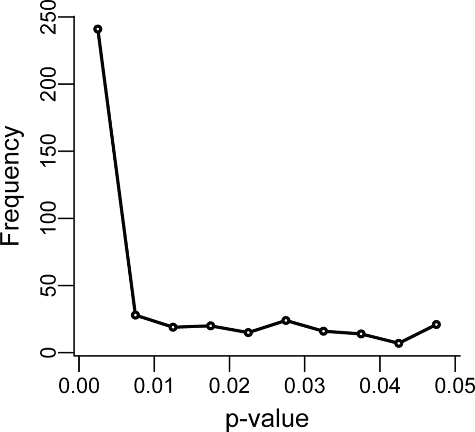
Head et al., PLOS Biology 2015, CC BY 4.0

• p < 0.05 meant to gauge evidence
• careers depend on clearing it
• researchers exploit “degrees of freedom”

. . .

a tell-tale excess of p-values just below 0.05

You met this in Chapter 10. The 0.05 threshold was a proxy for evidence strength; once publication depends on it, the literature shows a spike of p-values landing just under the line. The agent here is the researcher, gaming the threshold.

you have already seen Goodhart’s law

• Chapter 6: train loss falls while test loss rises
• a proxy (training loss) optimized so hard it stops tracking the goal (generalization)

same mechanism as VW and the hospitals, only the cast changes

• there: people adapt after the metric carries stakes
• in ML: the single agent is the learning algorithm, memorizing noise

This is the surprise. Overfitting is Goodhart’s law. The training-loss/test-loss divergence students saw in Chapter 6 is the same phenomenon as gaming readmission penalties and cheating emissions tests. The difference is just how many agents are gaming, and whether they’re people or an optimizer.

cross-validation resists it: partly

• separate train / validation / test
• use the test set once, after all decisions are locked

but tune enough against the validation set, and it stops measuring generalization

and ML sees only one side: real Goodhart is dynamic, agents respond after deployment

CV is the ML defense, and it works against the static version. The full law is dynamic: the data is generated by strategic agents who respond to the metric in deployment. No held-out set captures that.

game the metric

your hospital is paid on its 30-day readmission rate.

name a way to lower the measured rate without treating anyone better. what hidden check would catch you?

DISCUSSION: Think-pair-share (5 min). Think and jot; pair and compare; debrief into “the Goodhart question” slide next.

If stuck: “who decides whether a returning patient counts as ‘admitted’?”

Key insight: hold returning patients in observation status or treat-and-release in the ED — neither counts as a readmission, and the sickest patients are easiest to divert. This is exactly the documented HRRP gaming (Wadhera et al. 2018). A hidden audit metric — post-discharge mortality, or total post-discharge ED visits — catches what the readmission count misses. This is the live setup for the two Goodhart questions.

the Goodhart question

whenever a prediction drives a decision, ask:

1. can the agents move this metric without advancing the goal?
2. who’s best positioned to? are they who the policy meant to reward?

defenses:

• audit with a hidden second metric
• cap how often anyone updates against it
• randomize a holdout

If yes to (1), you have a Goodhart problem; if (2) names the wrong beneficiaries, an equity problem on top. The strongest defense — randomizing a holdout to see the unperturbed world — is causal inference, Chapter 19.

what to do

before deployment

• split by the right axis: time? person? ask what generalization you need
• simulate the deployed action: score what the prediction causes, not just the prediction
• audit proxy vs. outcome: write down the goal each metric stands for
• stress-test the tails: build out-of-distribution cases before deployment

Four habits. The second is the feedback-loop defense: models whose predictions drive decisions can’t be validated on passive historical data alone.

after deployment

• monitor drift: track performance against fresh ground truth
• hold out a control: a sample where the model doesn’t decide
• A/B test major changes: randomize to measure impact causally

A/B testing is the single most effective defense against feedback-loop failures

machinery: Chapter 19

When performance erodes, ask: did the world change, did the model change the world, or is the metric being gamed? The control shows what would have happened without the model. Chapter 19 develops the randomization machinery.

what we covered

• temporal leakage → walk-forward validation, not random splits
• distribution shift → no split fixes a regime you never saw
• feedback loops → randomized holdouts, not better splits
• WMD → unmeasurable + harmful + self-fulfilling
• Goodhart → metric becomes target; overfitting is the special case

Revisit the agenda. The through-line: match the validation procedure to the failure mode, and recognize when no procedure will help. Report prediction intervals, not point forecasts.

next: working with AI

we can build, validate, and stress-test models.

can AutoML and LLMs do this for us?

• Chapter 17: a 15-item checklist for any analysis
• items #13 (Goodhart) and #14 (feedback loops) point back here

Forward pointer. Chapter 17 is the synthesis — what AI tools do well, and the judgment they can’t replace. Two of its checklist items are exactly today’s deepest failure modes.

feedback

forms.gle/feedback

what worked? what didn’t? what’s still confusing?

Standard feedback slide. Same form as previous lectures.