Lecture 3: Data munging

Applied Statistics: From Data to Decisions

Professor Madeleine Udell

Monday, April 6, 2026

concept check from last time

df.describe() says the Airbnb price column has 3,818 values

df.shape says the DataFrame has 4,229 rows

Q: where did the other 411 rows go?

• .describe() silently skips NaN — 411 listings have missing prices
• always compare .describe() counts against .shape

Quick concept check, ~2 min. This tests the key EDA skill from lec02: notice when counts don’t match. The answer: .describe() drops NaN values from its count. 411 listings have no price. This is the EDA workflow in action: shape → types → distributions → missing data. It also sets up today’s lecture: “We noticed the missing data last time. Today we deal with it.”

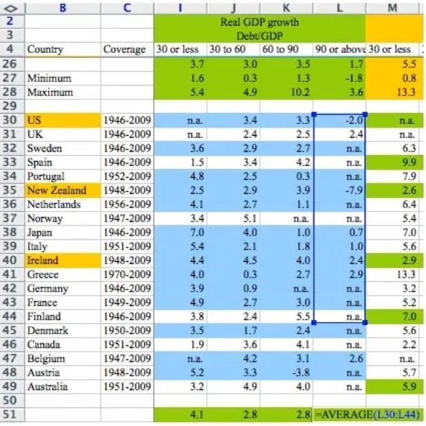
a cell range dragged one row too short. austerity budgets for millions of people.

Reinhart & Rogoff (2010) — Excel error discovered by Thomas Herndon, UMass Amherst

The hook. Carmen Reinhart and Kenneth Rogoff published a 2010 paper arguing GDP growth drops sharply when government debt exceeds 90% of GDP. This influenced austerity budgets across Europe and the US. Three years later, a grad student trying to replicate the results for a class assignment discovered an Excel formula selected only 15 of 20 countries — five were excluded because someone dragged a cell range one row too short. The corrected result: -0.1% growth became +2.2%. Show the chart — red bars are R&R original, blue bars are corrected. The “Above 90%” category is the entire basis for the austerity argument.

the spreadsheet

=AVERAGE(L30:L44) — but the data goes to row 49

Show the actual spreadsheet. The highlighted formula selects L30:L44 but the data continues to L49. Five countries — Australia, Austria, Belgium, Canada, Denmark — are excluded. The corrected average flips from -0.1% to +2.2%. A grad student found this trying to replicate results for a homework assignment. Pause and let students absorb: this error shaped fiscal policy.

three data disasters

Reinhart-Rogoff (2010)

cell range one row too short

→ austerity budgets for millions

Public Health England (2020)

.xls row limit: 65,536

→ 15,841 COVID cases lost, contacts never traced

gene naming (2016–2020)

SEPT1 → “1-Sep”

→ 20% of genomics papers corrupted, 27 genes renamed

all three are bugs — but in a spreadsheet, the bug is invisible

Three disasters, one pattern: each is a bug. A formula that selects the wrong range. A file format that truncates data. An auto-format that changes cell values. Bugs happen in any tool — the difference is whether you can find them. In a spreadsheet, the logic is hidden in cells. In code, every decision is a readable line.

why we write code

spreadsheets hide logic

• formula in cell G47 excludes rows
• dragged range stops one row short
• no one notices unless they click every cell

code makes decisions visible

• every drop, coerce, join is a readable line
• when wrong, the bug is findable
• when right, the logic is reproducible

good code is deterministic. same script, same data → same answer every time.

The Reinhart-Rogoff error was a formula hidden in a cell. The PHE error was an invisible row limit. Code makes every decision visible, reviewable, and reproducible.

AI analysis vs. AI-assisted code

	AI analyzes data directly	AI helps you write code
cleaning decisions	hidden	visible as lines you can read
reproducibility	different answers each session	deterministic
what you learn	nothing about the data	everything about the data

use AI to write code, not to replace understanding

This is the course philosophy. AI is a powerful tool for writing code. But uploading a CSV and asking for a summary skips the critical thinking. A 2025 study found ChatGPT gives inconsistent results on the same data — different factor structures, different conclusions, across sessions.

today’s concepts

every cleaning decision changes the answer

1. missing data — the many forms, MCAR / MAR / MNAR
2. joining datasets — inner vs. left, one-to-many
3. strings and deduplication — standardization, the birthday paradox
4. when tools betray you — handling missing data, coercion traps, AI-assisted code

Orient students. The thesis (“every cleaning decision changes the answer”) lands hard after the three disasters. Four sections, each about a place where a reasonable-seeming default produces a wrong answer.

recap: what we found last time

• Airbnb data: relatively tidy, NaN for missing values
• pandas handled it transparently: .isna(), .describe()
• but we noticed some dtypes looked wrong…

today: real datasets are rarely so cooperative

Brief recap, ~1 min. Connect to lec02 where students first saw the Airbnb data. The transition: “That was the easy case.”

1. the many faces of missing data

today’s dataset: College Scorecard

• US Department of Education
• 7,703 institutions, 122 columns
• SAT scores, enrollment, earnings, debt
• data dictionary, methodology, public updates

. . .

contrast: a random CSV on Kaggle with no documentation

Introduce the dataset. Emphasize provenance: this dataset has documentation, methodology, yearly updates. “Before you clean a dataset, ask where it came from.” The Scorecard is trustworthy because we can verify its methodology. A random Kaggle CSV? No way to know if it was collected, curated, or generated by an AI.

data provenance

data provenance

the chain of custody from data collection to your notebook

• documented methodology? ✓
• data dictionary defining every column? ✓
• known collection procedures? ✓
• public and versioned? ✓

in the AI era: synthetic datasets, undocumented web scrapes, training data contamination

Definition after motivation. Students just saw a concrete example of good provenance (Scorecard) and bad provenance (random Kaggle CSV). Now the definition lands.

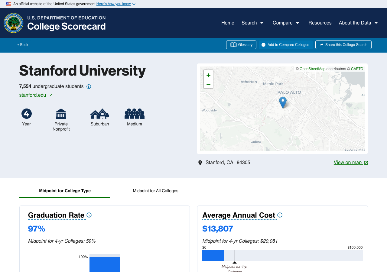
Stanford in the Scorecard

the Scorecard website says Stanford median earnings = $136,000 (4 years after completing)

but program-level data tells a different story:

program	credential	earnings (4yr)
Business Admin	Master’s	$262K
Computer Science	Master’s	$256K
Human Biology	Bachelor’s	$82K
English Literature	Bachelor’s	$82K
Ethnic Studies	Bachelor’s	$46K

$136K is a weighted average dominated by large graduate programs

This is the moment students connect personally. The Scorecard website says $136K, which sounds great. But that aggregate hides a 6x range: $46K to $262K. The aggregate is dominated by large programs and graduate degrees. Two caveats students should know: (1) only tracks Title IV aid recipients — many Stanford students pay without federal aid, so they’re invisible to the Scorecard. (2) Only 10 of Stanford’s 51 bachelor’s programs even report 4yr earnings — the rest have too few Title IV recipients. MS&E isn’t “PrivacySuppressed” — it’s simply absent, likely classified under “Engineering, Other” (CIP 1499, $115K) but there’s no way to confirm. The opaque CIP code mapping is itself a data quality problem.

navigating a data dictionary

the College Scorecard dictionary: 3,308 variables across 8 tabs

variable name	what it actually means
CONTROL	institution type: 1=Public, 2=Private nonprofit, 3=Private for-profit
MD_EARN_WNE_P10	median earnings of students working and not enrolled, 10 years after entry
PREDDEG	predominant degree: 0–4 coded as integers, but the values are categories
OPEID	defined as a string — store as integer and you lose leading zeros

CONTROL = 2 looks numeric. mean(CONTROL) = 1.7. what does that mean?

Show the actual Excel file briefly — 3,587 rows, 14 columns, 8 tabs. The point: variable names are cryptic, coded integers look numeric but aren’t, and you can’t skip the dictionary. _P10 means “pool 10 years after entry,” not 10th percentile. CONTROL is a category encoded as integers. The dictionary is the only way to know. ~2 min.

a column that should be numeric

MD_EARN_WNE_P10 — median earnings, 10 years after entry (working and not enrolled)

dtype: str

Q: why would an earnings column be stored as a string?

Pause after showing the dtype. Let students guess. Common answers: “formatting”, “dollar signs”. The real answer is more interesting.

the culprit: PrivacySuppressed

Non-numeric values in 'MD_EARN_WNE_P10':
PrivacySuppressed    480

• a string sitting in a numeric column
• cohort too small → Department of Education suppresses data to protect privacy
• pandas treats the whole column as str

This is the first “aha” — a single string value in 480 rows forces the entire column to be non-numeric. Every arithmetic operation, every plot, every model will fail or give wrong results.

the missingness zoo

encoding	where you’ll find it	pandas detects it?
NaN, None	standard pandas	yes
"" (empty string)	CSV exports	no
"N/A", "NA"	manual data entry	sometimes
"PrivacySuppressed"	government data	no
-999, 99, 0	sensors, surveys	no
absent rows	panel/time-series	no rows to detect

chapter 2 covered row 1. everything else requires active detection.

Show the full zoo. The key point: NaN is the easy case. Most missingness hides in plain sight.

why categories are stored as integers

CONTROL: 1 = Public, 2 = Private nonprofit, 3 = Private for-profit

why not store the string?

• "Management Science and Engineering" = 37 bytes
• 7 = 1 byte

across 7,703 rows × hundreds of columns, integer codes cut storage by 10–50×

the tradeoff: you need the data dictionary to know what the numbers mean

This is the engineering reason behind integer encoding. Every categorical variable in the Scorecard is stored as an integer: CONTROL (institution type), PREDDEG (predominant degree), LOCALE (urbanicity), CCBASIC (Carnegie classification). The “Management Science and Engineering” example is from the field_of_study file where program names ARE stored as strings — and that file is 10× larger than the institution file as a result. The Scorecard designers made a deliberate choice: store codes, publish a dictionary. The danger: if you lose the dictionary, CONTROL = 2 is meaningless. And mean(CONTROL) = 1.7 is nonsense arithmetic on a category.

Demo: College Scorecard exploration

open in Colab

Switch to notebook. Show: load data with pd.read_csv, check dtypes.value_counts(), find non-numeric values in MD_EARN_WNE_P10, count PrivacySuppressed across all columns (7 columns affected). ~5 min.

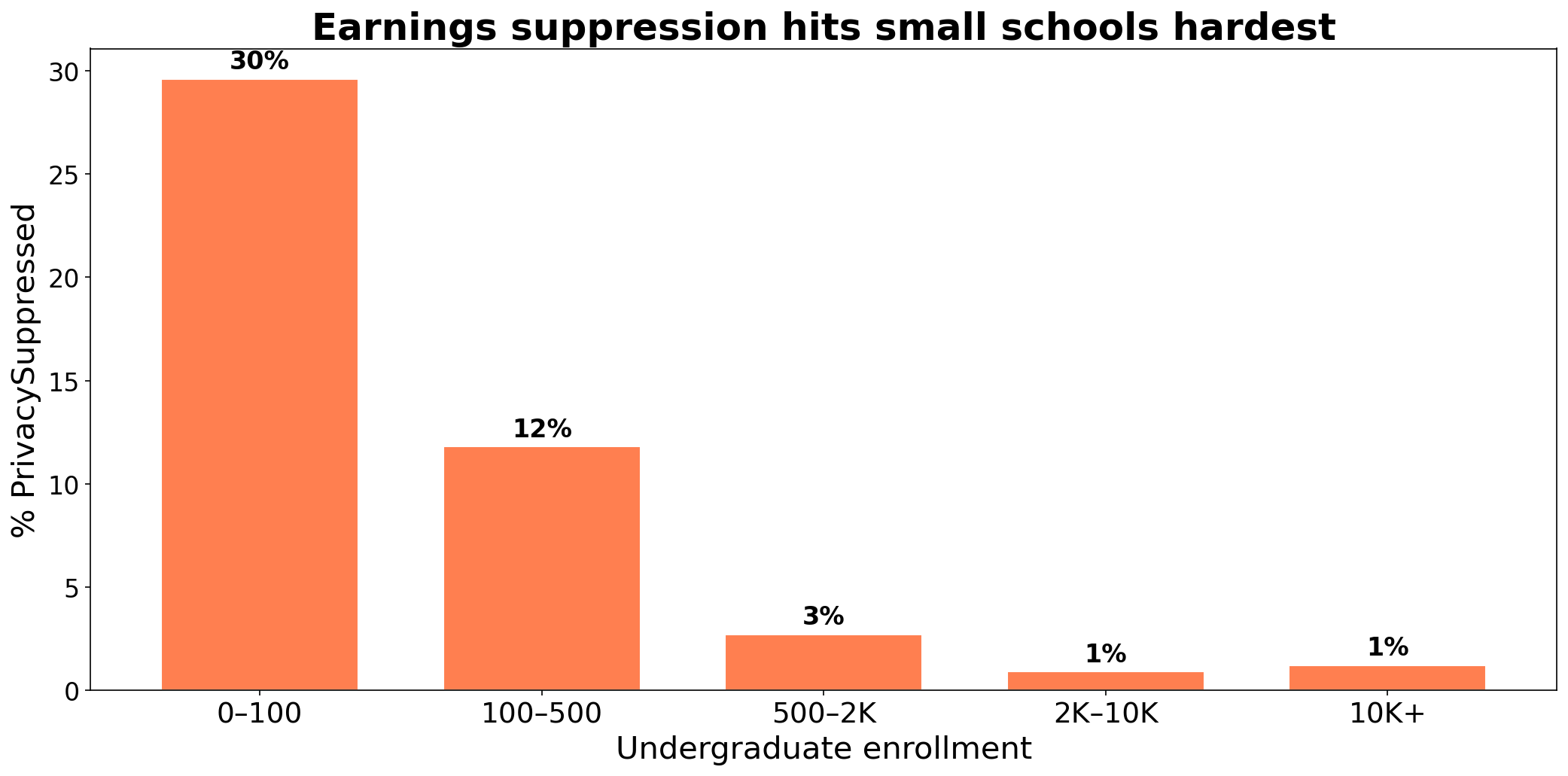
missingness is not random

Show the bar chart from the book: suppression rate by school size. Nearly a third of the smallest schools have suppressed earnings; among 2K+ schools, it’s about 1%. Lead with the evidence before the definitions.

three patterns of missingness

MCAR / MAR / MNAR

• MCAR: no pattern — mold destroys random records
• MAR: depends on observed data — SAT scores missing because school doesn’t require them (degree type is recorded)
• MNAR: depends on the missing value itself — sickest patients don’t report

College Scorecard earnings: MNAR

small cohort → suppressed → small schools are systematically different

Define the three patterns. The SAT example: certificate programs (cosmetology, truck driving) don’t require SATs, so SAT_AVG is missing. Missingness depends on degree type (PREDDEG), which we observe — that’s MAR. MNAR is the hardest — no observed variables can fully correct for it.

classify each scenario as MCAR, MAR, or MNAR:

1. a lab assistant drops a tray; 12 random blood samples are destroyed
2. SAT scores are missing for most certificate programs in the Scorecard
3. College Scorecard suppresses earnings when the cohort is too small

DISCUSSION: Classification exercise (4 min — 1 min individual, 1 min compare, 2 min class). Answers: (1) MCAR — the breakage is unrelated to any variable. (2) MAR — missingness depends on degree type (PREDDEG), which we observe. Certificate and associate programs don’t require SATs. (3) MNAR — small cohort → suppressed. But small cohort size is itself outcome-related: schools where fewer graduates are working may have worse earnings. If stuck: “Ask yourself: does the reason for missingness depend on the missing value itself?” Key insight: Only MNAR is truly dangerous — no observed variable can fully correct for it.

data leakage

suppose you want to predict graduation rate from admission data

the Scorecard has COMP_ORIG_YR4_RT (4-year completion rate) and MD_EARN_WNE_P10 (earnings 10 years later)

if you include earnings as a predictor of graduation… you’re using the future to predict the past

data leakage

when your model accidentally sees information from the future or the target variable

Leakage is easy to spot in this dataset. Earnings are measured 10 years after entry — using them to predict graduation (measured 4 years after entry) is using the future to predict the past. The Scorecard has many variables measured at different time points, making leakage tempting: retention rate (1yr), completion rate (4yr), earnings (10yr), debt (various). A model trained with leaked features looks great on training data and fails in production. The defense: for every variable, ask “when was this measured?” and “would I have this information at prediction time?”

2. joining datasets

why join?

the Scorecard comes in two files:

• scorecard.csv — one row per institution (SAT, enrollment, earnings)
• field_of_study.csv — one row per school-program pair (earnings by major)

richer questions require combining tables

• “do engineering programs pay more than humanities at the same school?”
• “should I take on more debt for a prestigious school?”

Motivate joins with a real question students care about. Two files, one question that requires both. ~1 min.

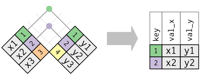
joining = matching rows by a shared key

pd.merge(left, right, on='key')    # match rows where key values agree

two flavors:

• inner join — keep only rows with a match in both tables
• left join — keep every row from the left table; fill NaN where no match exists

One-sentence definitions before the toy example. Students need the vocabulary to answer the prediction question on the next slide. ~30 sec.

inner join vs. left join: a toy example

Students

student	major_id
Alice	101
Bob	102
Carol	103

Majors

major_id	major_name
101	Physics
102	English
104	History

Q: which students survive an inner join on major_id?

Show both tables. Pause and ask students to predict. Carol (103) has no match in Majors. History (104) has no match in Students. Students now have the definition from the previous slide.

inner join: only matching rows

Inner join result

student	major_id	major_name
Alice	101	Physics
Bob	102	English

• Carol is gone (no match for 103)
• History is gone (no match for 104)
• only IDs in both tables survive

diagram: Wickham & Grolemund, R for Data Science

Reveal the result. Emphasize: inner join silently drops rows. Carol disappears and pandas doesn’t warn you. The R4DS diagram on the right shows the same idea with colored keys — matching keys (1, 2) are kept, non-matching keys (3, 4) are dropped.

left join: keep all left rows

Left join result

student	major_id	major_name
Alice	101	Physics
Bob	102	English
Carol	103	NaN

• all three students survive
• Carol’s major becomes NaN (no match)
• History still dropped (not in left table)

Left join preserves all rows from the left table. The NaN is a signal — “this student has no matching major.” That signal is lost in an inner join.

one-to-many: row multiplication

Left (2 rows)

left_id	key
L1	A
L2	A

Right (3 rows)

key	right_val
A	X
A	Y
A	Z

. . .

Result: 2 × 3 = 6 rows

left_id	key	right_val
L1	A	X
L1	A	Y
L1	A	Z
L2	A	X
L2	A	Y
L2	A	Z

every key matches → inner join = left join here. the difference only shows when keys are missing.

This is the key surprise. Joins can GROW your data, not just shrink it. 2 left rows × 3 right matches = 6 output rows. Since every key in the left table appears in the right table, inner and left join give the same result here — the distinction only matters when some keys are unmatched. This is intentional when joining institutions to programs — but a disaster when you think the key is unique and it isn’t.

defense: check your key before joining

assert scorecard['UNITID'].is_unique, \
    "UNITID is not unique — join will multiply rows!"

an assert that passes is documentation

an assert that fails is an alarm

This is a critical habit. One line of code prevents the most common join disaster. The assert pattern generalizes: after every cleaning step, assert what you expect.

• scorecard: 7,703 institutions
• programs: 228,000 rows across 5,500 institutions
• predict: how many rows will the inner join produce?
• more or fewer than 7,703?

DISCUSSION: Predict-then-reveal (5 min — 1 min think, 2 min share, 2 min class). If stuck: “Each institution matches to many programs. Stanford alone has 180+ programs.” Key insight: The inner join produces ~216,000 rows — a massive expansion because each institution is replicated once per program. Students who predicted “fewer” were thinking about inner joins as filters. The join is one-to-many.

Demo: join explosion

open in Colab

Switch to notebook. Show: pd.merge(scorecard, programs, on='UNITID', how='inner'), the row explosion (7K → 216K), the left join preserving all scorecard rows, the row count bar chart. Compare inner vs left. ~5 min.

after every join: check row counts

print(f"Scorecard rows:  {scorecard.shape[0]:,}")
print(f"Inner join rows: {inner.shape[0]:,}")
print(f"Left join rows:  {left.shape[0]:,}")

	gained rows?	lost rows?	what happened?
inner	yes (one-to-many)	yes (unmatched keys)	both at once
left	yes (one-to-many)	no	NaN for unmatched

the join type is a decision, not a default

Reinforce the key principle. Neither join type is “right” — each gives a different answer, and the choice should be deliberate.

3. strings and deduplication

string standardization

scorecard['INSTNM'].value_counts().head()

University of Phoenix-Arizona          1
University Of Phoenix-Arizona          1
UNIVERSITY OF PHOENIX - ARIZONA        1

scorecard['INSTNM_clean'] = (scorecard['INSTNM']
    .str.lower()
    .str.strip()
    .str.replace(r'\s+', ' ', regex=True))

lowercase → strip → collapse whitespace. every merge and groupby depends on this.

The Scorecard data is relatively clean, but messy string data is the norm. Show the three variants of U of Phoenix. Without standardization, groupby treats these as three different schools. The .str accessor is the pandas tool for string cleaning. ~2 min.

quick poll: voter registration

• ✋ who is registered to vote here (Santa Clara County)?
• ✋ who is registered at home (where your parents live)?
• ✋ who canceled their previous registration when they registered here?
• ✋ who plans to vote here? there? …both places?

Hands-up poll, ~1 min. Most students will be registered in two states. Almost no one will have canceled the old registration. No one will admit to voting twice (laugh). The point: you are a “duplicate” in the national voter file. This makes the next slide personal.

when is a duplicate not a duplicate?

US voter registration: 104 million records across 50 states

match on name + date of birth → 761,875 apparent duplicates

Q: are these really the same person?

Goel, Meredith, Morse, Rothschild & Shirani-Mehr, “One Person, One Vote,” APSR 2020

Transition from joins to deduplication. Source: Goel et al., “One Person, One Vote: Estimating the Prevalence of Double Voting in U.S. Presidential Elections,” American Political Science Review, 2020. 104M voter records from the 2012 election, 762K name+DOB matches. Sounds like massive fraud — but is it?

the birthday paradox strikes

suppose 141 voters named “John Smith” were born in 1970

• expected matching-birthday pairs: \(\binom{141}{2} \times \frac{1}{365} \approx 27\)

• that’s 27 “double voters” — from one common name in one birth year

scale this across every name in the country: most of those 762K matches are coincidences

The John Smith example is stylized to illustrate the mechanism. The paper’s actual method: model the birthday distribution for each name (accounting for day-of-week, seasonal, and name-specific patterns like “June” clustering in June), compute expected coincidental matches across all name groups, and subtract. Result: 97% of the 762K matches are two distinct people who happen to share a name and birthday. The estimated number of actual double votes: ~21,000 before measurement error, and possibly near zero after accounting for clerical errors in poll books. Canceling registrations based on name+DOB matches would disenfranchise over 300 legitimate voters per double vote prevented.

deduplication is a value judgment

• merge too aggressively → remove legitimate distinct records
• merge too conservatively → count the same entity twice

in the voter file: canceling registrations by name+DOB match would disenfranchise 300+ legitimate voters per double vote prevented

the same tradeoff appears everywhere:

• patient records across hospitals
• customer records across systems
• College Scorecard branch campuses (same OPEID6, different UNITID)

The 300:1 ratio is from the paper — based on Iowa Crosscheck data where SSN verification revealed that fewer than 10 of 26,000 confirmed duplicate registrations involved both records being used to vote, while 2,500+ cases had the earlier-dated registration used to cast a legitimate vote. Connect back to the Scorecard. University of Phoenix has dozens of UNITIDs but one OPEID6. Whether you treat them as one institution or many depends on your question.

4. when tools betray you

three approaches to missing earnings

same question: “what is the average median earnings?”

approach	method	mean	side effect
drop rows	dropna(subset=['earnings'])	$42,290	removes schools from all columns
fill with mean	fillna(mean_val)	$42,290	shrinks std, distorts correlations
ignore NaN	pandas default (.mean() skips NaN)	$42,290	preserves full DataFrame

same mean — but dropping rows changes which schools remain in your sample

~3 min. The mean is identical by construction (mean imputation preserves the mean; dropping rows computes the mean over the same non-missing values). The damage is elsewhere: dropping rows removes those schools from ALL columns, biasing every downstream analysis. Mean imputation shrinks the standard deviation and distorts correlations. “Ignore NaN” is pandas’ default and the least harmful for a single column, but still masks the missingness pattern. The next slide shows the real problem.

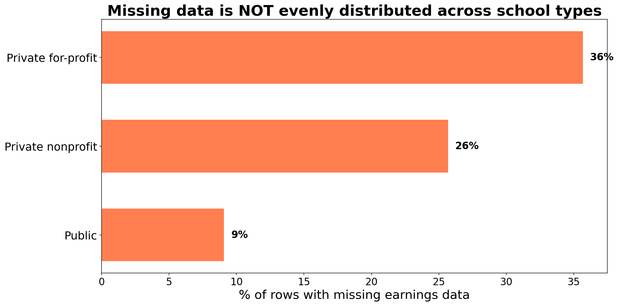
the damage shows in group comparisons

dropping rows with missing earnings changes which schools remain

Show the bar chart: % missing by school type. For-profit schools have far more missing data. Drop those rows and your “cleaned” dataset is biased toward public and nonprofit schools. This is informative missingness — the absence of data tells you something about the institution.

an AI assistant “cleans” the College Scorecard by calling .dropna()

• it reports the average earnings is $45,000
• name two questions you’d ask before trusting that number
• focus on what was lost in the cleaning step

DISCUSSION: Think-pair-share (7 min — 2 min think, 3 min pair, 2 min class). If stuck: “How many rows survived? Which types of schools were dropped? What was the missingness rate?” Key insight: The questions to ask are: (1) how many rows did you drop? (2) are the dropped rows systematically different? (3) which approach did you use and why? This is the critical evaluation skill.

when coercion erases distinctions

imagine an income column with these non-numeric values:

value	meaning
"PrivacySuppressed"	cohort too small
">100,000"	top-coded (Census)
"<LOD"	below limit of detection
"Refused"	survey respondent declined
"N/A"	question didn’t apply

pd.to_numeric(errors='coerce') turns all five into NaN

five different reasons for missingness → one undifferentiated blank

This is the real problem with errors=‘coerce’: not that it creates NaN (NaN is fine when you expect it), but that it collapses multiple DISTINCT reasons for missingness into a single indistinguishable value. “PrivacySuppressed” means small cohort. “>100,000” means the value is KNOWN to be high but capped. “Refused” means the person actively withheld. These carry very different implications for analysis. After coercion, all that context is lost. The defense: always run value_counts() BEFORE coercing, so you know what you’re erasing.

sentinel values

-999 and 999999 aren’t missing — they’re wrong

Mean WITH sentinels:    -208.6°F
Mean WITHOUT sentinels:   72.9°F

unlike NaN, sentinel values participate in every computation without warning

Quick example. A temperature sensor records -999 when it malfunctions. The mean is wildly wrong, and nothing raises an error. The only defense: know your data dictionary, check for impossible values.

the identifier trap

OPEID 00102100 → stored as integer → becomes 102100

• leading zeros vanish
• later join against zero-padded strings: zero matches, no error

ZIP codes, phone numbers, IDs — codes, not numbers

Quick point. Identifiers that look like numbers but aren’t. Arithmetic on them is meaningless. Storing them as integers loses leading zeros and breaks downstream joins.

this code merges two tables and computes mean earnings. it has at least four bugs.

merged = pd.merge(scorecard, programs, on='UNITID')
mean_earn = merged['EARN_MDN_4YR'].mean()

find as many as you can. for each, explain what goes wrong and how to fix it.

DISCUSSION: Analyze-this (5 min — 3 min small groups, 2 min share-out). Correct answers — at least four problems: (1) No how= specified — defaults to inner join, silently dropping unmatched schools. (2) No assert on key uniqueness — one-to-many join will replicate institution rows, inflating the mean toward schools with many programs. (3) No pd.to_numeric(errors='coerce') — EARN_MDN_4YR contains strings (PrivacySuppressed, blanks) that block .mean(). (4) No check of how many rows survived — could be computing mean from a biased subset. Bonus: the join includes all credential levels (Bachelor’s through Doctoral), mixing very different populations. If stuck: “What kind of join is this? How many rows will it produce?”

data munging checklist

1. check provenance — where did the data come from?
2. check types — any str columns that should be numeric?
3. find the missing data — NaN, sentinels, string placeholders, absent rows
4. understand why data is missing — MCAR, MAR, MNAR?
5. check joins — row counts after every merge. assert.
6. standardize strings — lowercase, strip, collapse variants
7. verify type conversions — how many values became NaN?
8. compare groups — is missingness evenly distributed?

This is the checklist from the book. Students should internalize this as a workflow they run every time they encounter a new dataset. Each item connects to a concrete example from today’s lecture.

“the combination of some data and an aching desire for an answer does not ensure that a reasonable one can be extracted from a given body of data.”

— John Tukey

Let this sit for a moment. The quote captures the entire lecture: cleaning decisions matter, tools can betray you, and any analysis produces something — but something is not the same as something correct. John Tukey (1915-2000) was one of the most influential statisticians of the 20th century — he coined “bit”, invented the FFT algorithm with Cooley, and pioneered exploratory data analysis.

synthesis

1. missing data hides in many forms — NaN is just the easy case; MNAR is the dangerous one
2. joins can grow or shrink your data — check row counts after every merge
3. strings and deduplication — standardize before matching; the birthday paradox generates false positives at scale
4. tools betray you — coercion erases distinctions, dropping rows changes the sample, code makes every decision visible

Revisit the agenda items with takeaways. Each bullet maps to a content block. This is the “what you should remember” version of the lecture.

next time: linear algebra

we can clean and join data. now we need a language for modeling it.

• vectors as data points, vectors as features
• linear combinations → predictions
• span → what a model can reach

preview: Chapter 4 in the course notes

Forward pointer. “We’ve spent two lectures getting data ready. Now we build the mathematical machinery to do something with it.” The transition from Act 1 data prep to Act 1 modeling.

before next class

• fill out the homework discussion section scheduling survey (see Ed)
• read Chapter 3 in the course notes
• try the notebook exercises on your own
• Quiz 1 is Wednesday — covers Lectures 1-3. be on time!

one-minute feedback

1. what was the most useful thing you learned today?
2. what was the most confusing?

give feedback

Last 1-2 minutes. Anonymous. QR code goes to the same form. Entry field pre-filled with “3” for lecture number.