Lecture 15: Clustering — K-Means

MSE 125 — Applied Statistics

Madeleine Udell

Monday, May 18, 2026

logistics

  • HW 4 out — HMDA Kaggle challenge, due Mon May 25
  • Quiz 7 Wed May 20 — PCA + clustering
  • project midterm returned this week

the brief

Pacers front office

goal: sign a wing who can space the floor and attack closeouts

the five-position label is no help — Curry and Westbrook are both “point guards” and play nothing alike

what is the real taxonomy of NBA players in 2024?

today

  • k-means — assign, recompute, repeat
  • choosing k, checking stability — what the standard tools tell you (and what they don’t)
  • your features pick your clusters — and that’s the whole game
  • four published case studies — when clustering works and when it doesn’t

bridge from PCA

PCA k-means
structure found directions of variance groups of rows
representation continuous (low-dim coords) discrete (one label per row)
standardize first yes — distances depend on units yes — same reason
labels needed no no

both are unsupervised. PCA compresses; k-means partitions.

317 players, five court zones

the data

shot-attempt counts from the 2023-24 NBA regular season

filter to players with ≥ 200 FGA → 317 players

for each player, the share of attempts in five court zones:

  • RA — restricted area (right at the rim)
  • PAINT — non-restricted paint
  • MID — midrange
  • C3 — corner three
  • ATB3 — above-the-break three

the five shares sum to 1 — a shot-mix fingerprint

what does “similar” mean?

before any algorithm runs, we commit to a notion of distance

Euclidean distance (on standardized shot mix)

d(x_i, x_j) = \sqrt{\sum_{z=1}^{5} (x_{iz} - x_{jz})^2}

square the differences zone by zone, add, square-root

two players are “close” when their five shot shares line up — regardless of height, defense, rebounding, or total volume

famous pairs

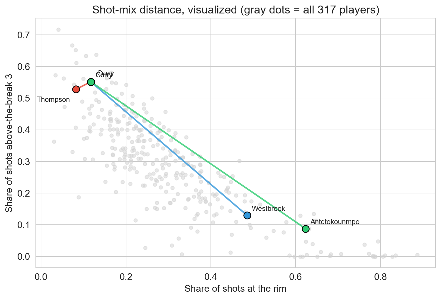
gray dots = all 317 players. colored lines = three famous pairs in shot-mix distance.

assign, recompute, repeat

k-means in three steps

k-means clustering

partition n points into k groups by repeating:

  1. initialize k centroids (randomly)
  2. assign each point to the nearest centroid
  3. recompute each centroid as the mean of its assigned points

loop on 2-3 until assignments stop changing

  • centroid — the mean of all points in a cluster
  • converges in finite steps (finitely many assignments; SSE only goes down)
  • the solution is a local optimum, not necessarily the global one

watch it iterate

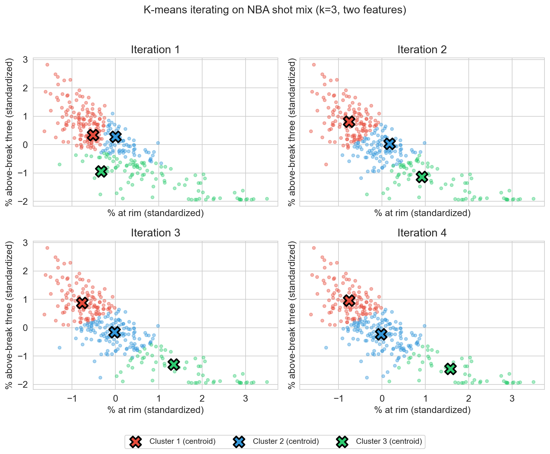
k=3, two features (rim share, above-break-3 share), four iterations
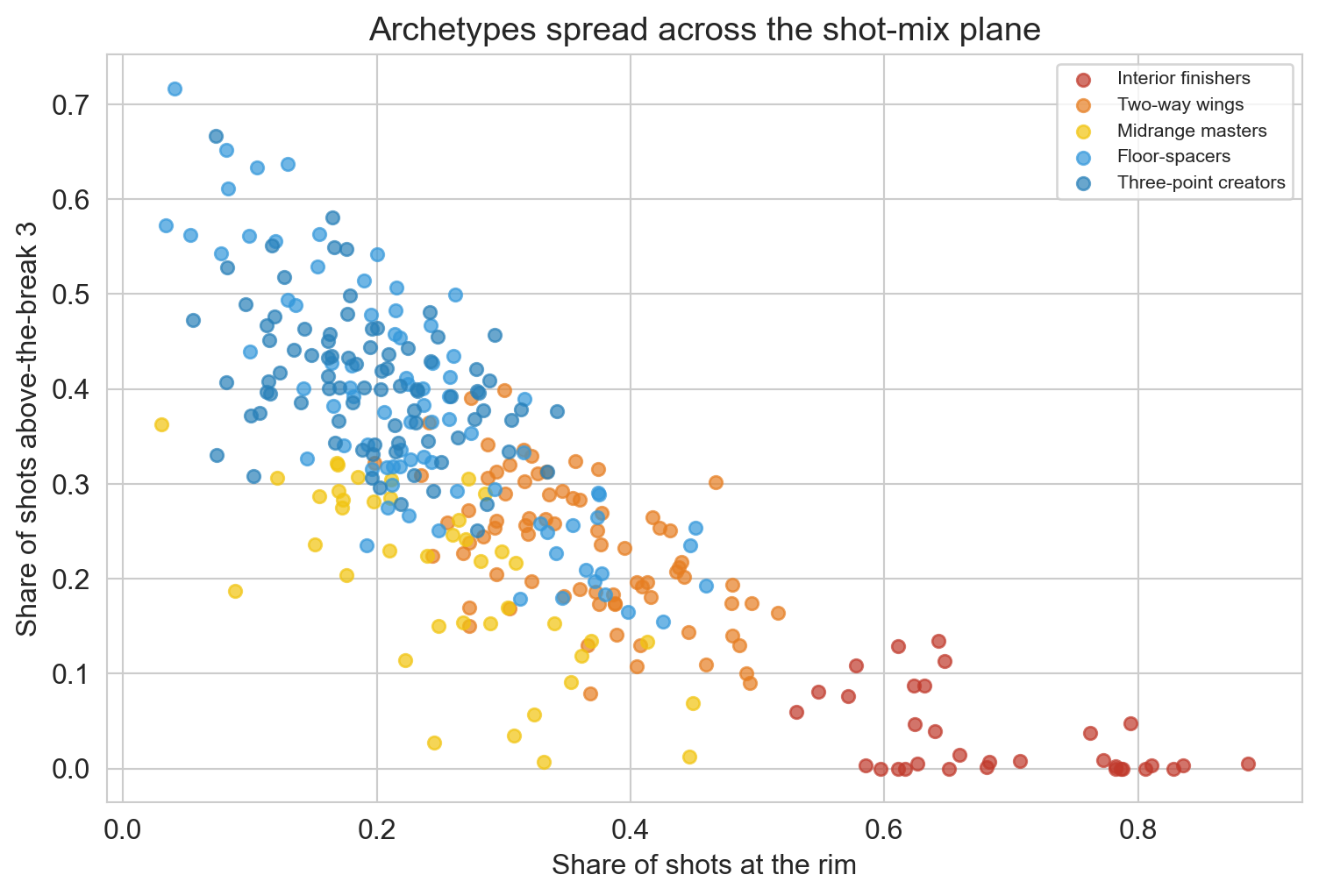
the objective

sum of squared errors (SSE)

\text{SSE} = \sum_{k=1}^{K} \sum_{i \in C_k} \|x_i - \mu_k\|^2

total squared distance from each point to its assigned centroid

  • C_k = set of points assigned to cluster k
  • \mu_k = centroid of cluster k (the mean of those points)
  • same form as regression SSE — “prediction” for x_i is its cluster’s centroid

alternating minimization — same engine as PCA in Ch 14

one more thing first — standardize

k-means uses Euclidean distance

→ a feature with range 0-1000 dominates one with range 0-1

even when shot shares already sum to 1, standardize before clustering — safe default for any distance-based method

same lesson as PCA: standardize before any distance-based method

run it — all five zones

features = ['pct_RA', 'pct_PAINT', 'pct_MID', 'pct_C3', 'pct_ATB3']

X = StandardScaler().fit_transform(nba[features].values)

kmeans = KMeans(n_clusters=5, random_state=42, n_init=10)
labels = kmeans.fit_predict(X)
Cluster sizes: {0: 54, 1: 76, 2: 67, 3: 60, 4: 60}

five clusters, sizes 54-76. what’s in each?

five archetypes

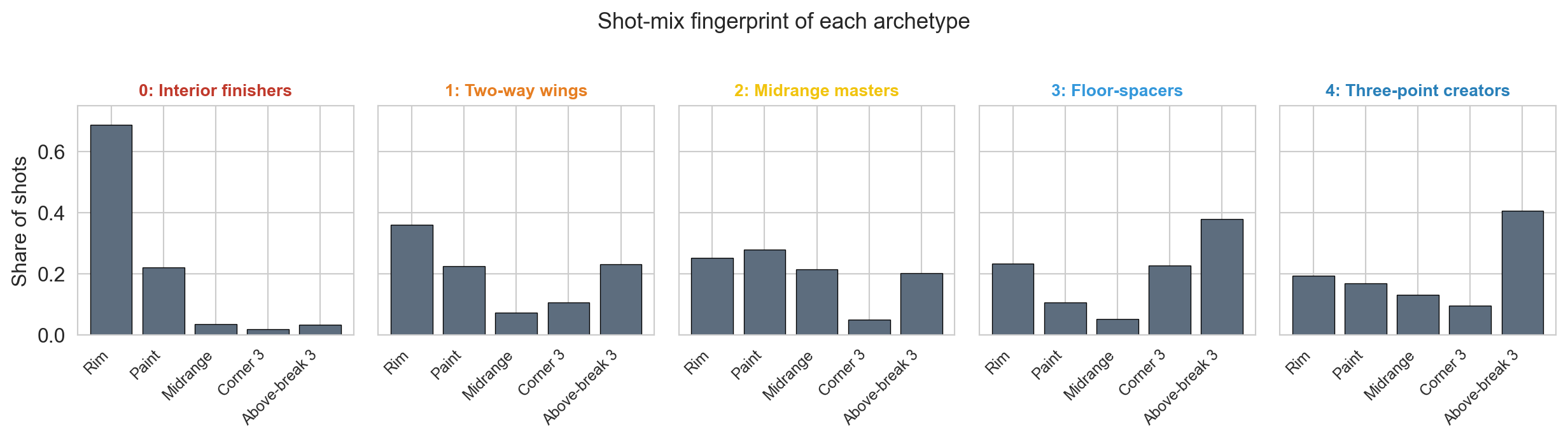
each panel = one archetype’s mean shot mix across the five zones

the archetypes spread across the floor

k-means didn’t see position labels at all — yet the midrange-masters cluster mixes a guard (Brunson), a wing (Edwards), and a forward (Durant).

one iteration of k-means — on paper.

four points: (0, 0), (1, 0), (4, 3), (5, 3).

two initial centroids: \mu_1 = (1, 1), \mu_2 = (3, 2).

  1. assign each point to its nearest centroid (Euclidean).
  2. recompute each centroid as the mean of its assigned points.

what are the new centroids?

how do you pick k?

elbow + silhouette: the standard tools

elbow method

plot SSE vs. k; look for a bend where adding clusters stops helping

silhouette score

for each point, s(i) = \dfrac{b(i) - a(i)}{\max(a(i), b(i))} \in [-1, 1]

  • a(i) = mean within-cluster distance
  • b(i) = mean distance to nearest other cluster

near +1 = sits comfortably in its cluster, 0 = on a boundary, -1 = probably misassigned

what do the heuristics say?
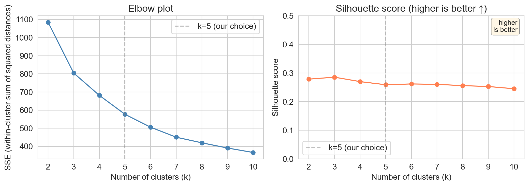
  • elbow — gradual, no sharp bend
  • silhouette — peaks at k=3 (k=2 a close second), then drifts down
  • both rule out clearly bad k, neither picks k for you

silhouette, per player

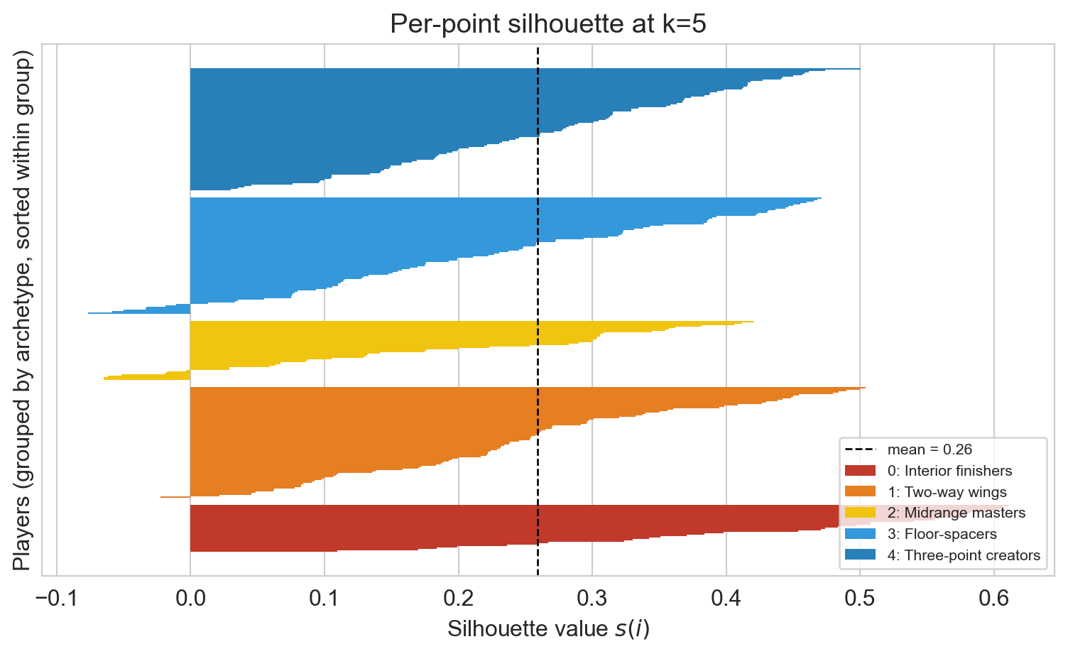
each bar = one player’s silhouette score, grouped by archetype

silhouette says k=3. we picked k=5. why?

what information did we use that the silhouette score does not see?

k=3

three coarse buckets — bigs, wings, guards

k=5

five archetypes — finishers, wings, midrange, spacers, creators

don’t commit to k up front

hierarchical clustering: don’t commit to k up front

if the right k is unclear — build a tree instead

agglomerative hierarchical clustering

  1. start with every point as its own cluster
  2. merge the two closest clusters
  3. repeat until one cluster remains

cut the tree at any height → clustering at that granularity

a tree of merges

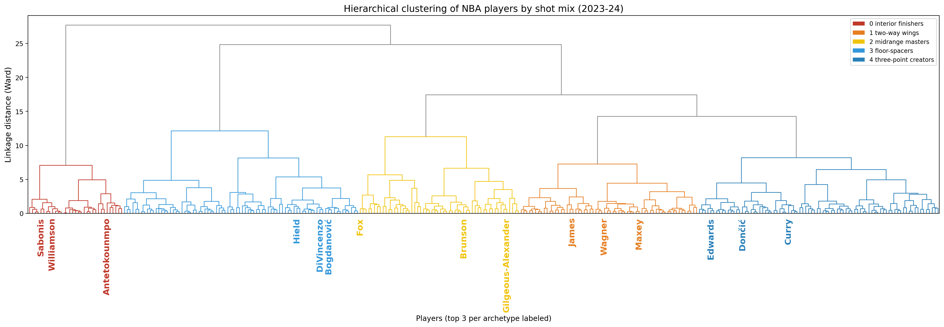
top 3 players by FGA in each archetype labeled. neighboring leaves play similarly.

  • cut high → coarse partition (a few big groups)
  • cut low → fine partition (many small groups)
  • a second algorithm on the same data — how much does it agree with k-means?

how stable is any of this?

comparing two clusterings

two clusterings of the same n points — how much do they agree?

Rand index (RI)

for every pair of points, the two clusterings either agree or disagree:

  • TP — both put the pair together
  • TN — both put the pair apart
  • FP / FN — one says together, the other says apart

\text{RI} = \frac{\text{TP} + \text{TN}}{\text{all pairs}}

adjusted Rand index (ARI)

RI inflates by chance — most pairs are “apart” under any partition. ARI corrects for that.

  • \text{ARI} = 1 → identical clusterings
  • \text{ARI} = 0 → no better than random
  • \text{ARI} < 0 → worse than random (rare)

different seeds, different clusters

k-means picks random initial centroids → different starts can converge to different local optima

we run k-means 10 times at k=5 with n_init=1 — how often do they agree?

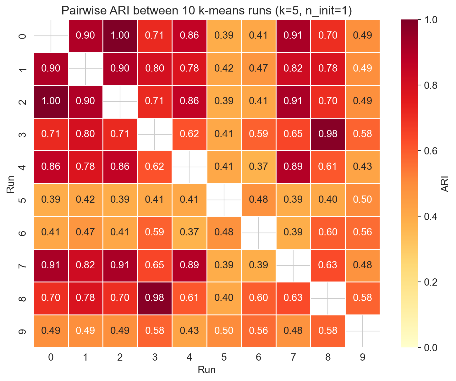
10 runs, pairwise ARI

  • mean ARI = 0.62, range 0.37 – 1.00 across 45 pairs
  • some pairs agree perfectly (ARI = 1); some find genuinely different partitions
  • same data, same algorithm, same k — different clusters across runs

sklearn’s defenses (and what they don’t fix)

# sklearn defaults:
KMeans(n_clusters=5, n_init=10, init='k-means++')
  • n_init=10 — runs k-means 10 times, keeps the lowest-SSE partition
  • k-means++ — picks initial centroids spread apart, not just random rows
  • together: most pairs of runs now agree closely; a few still diverge
  • cluster IDs are arbitrary — Cluster 3 in one run is Cluster 0 in the next
  • describe clusters by profile, not by integer label
  • boundary players flip across seeds — that’s signal, not noise: they’re hybrids sitting between archetypes

your features pick your clusters

same players, three feature sets

we have 317 players and k=5 in all three runs

shot mix

pct_RA, pct_PAINT,
pct_MID, pct_C3,
pct_ATB3

→ archetypes

shot volume

FGA (one feature)

→ tiers: stars to bench

shot efficiency

efg_pct (effective FG%)

→ tiers: skill ladder

same data, same k, same algorithm. three different stories.

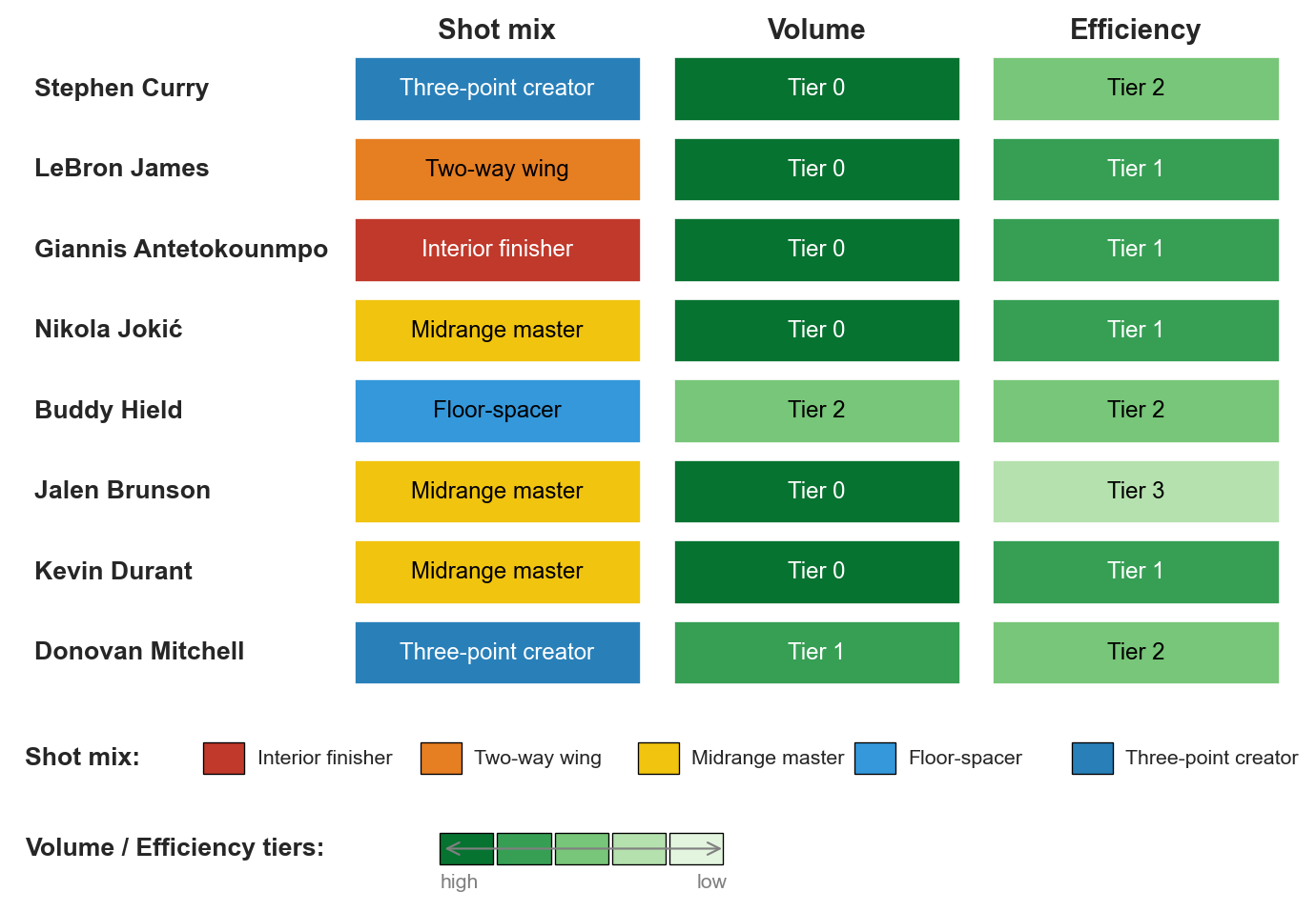
three stories, eight spotlight players

each row = one player labeled three ways. color encodes the tier.

features scramble clusters more than seeds do

three sources of disagreement, ranked by ARI:

  • across seeds — 10 k-means runs at k=5: mean ARI ≈ 0.62
  • across algorithms — k-means k=5 vs. hierarchical k=5: ARI ≈ 0.57
  • across feature sets — shot mix vs. volume / shot mix vs. efficiency / volume vs. efficiency: ARI ≈ 0

feature choice scrambles the partition an order of magnitude more than the random seed or the algorithm does

which clustering for which question?

  • GM looking for a Hield replacement → cluster on shot mix (find players who fill the same role)
  • GM ranking trade targets by raw production → cluster on volume (find players who do the same amount)
  • GM valuing a contract → cluster on efficiency (find players who score well per attempt)

there’s no “true” clustering of these players. each recipe answers a different question; the analyst picks which question the clustering should answer.

four cases from the literature

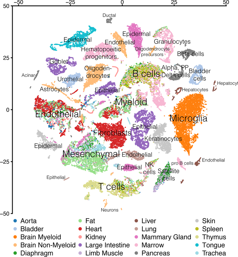
clustering as the scaffolding of a cell atlas

  • 100,605 mouse cells, 20 organs, no labels
  • PCA + graph clustering → ~50 clusters
  • each cluster annotated by its marker genes — decades of cell biology
  • almost every named cell type came back out
  • validation came from outside the algorithm

Tabula Muris Consortium, Nature 2018, Fig. 2

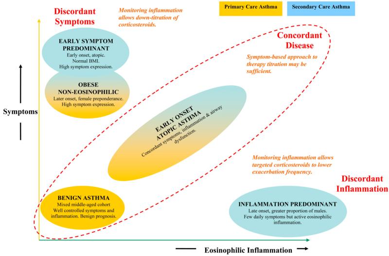
clusters that change which drug you should take

  • 184 + 187 + 68 asthma patients, 8 clinical features
  • hierarchical + k-means → 4 clusters
  • one cluster is discordant: high inflammation, few symptoms
  • RCT: treat by inflammation → exacerbations 3.53 → 0.38/yr (p = 0.002)
  • cluster membership predicted which treatment helped

Haldar et al., Am. J. Respir. Crit. Care Med. 2008, Fig. 1

beautiful clusters, no replication

  • Drysdale 2017, Nature Medicine. n = 1,188 depressed patients
  • CCA + hierarchical → 4 depression biotypes, 82–93% accuracy
  • Dinga 2019 replication, n = 187: permutation p of canonical correlations 0.64, 0.99
  • cluster p = 0.45. cross-validated correlations ~0
  • noise made visible by an under-regularized projection

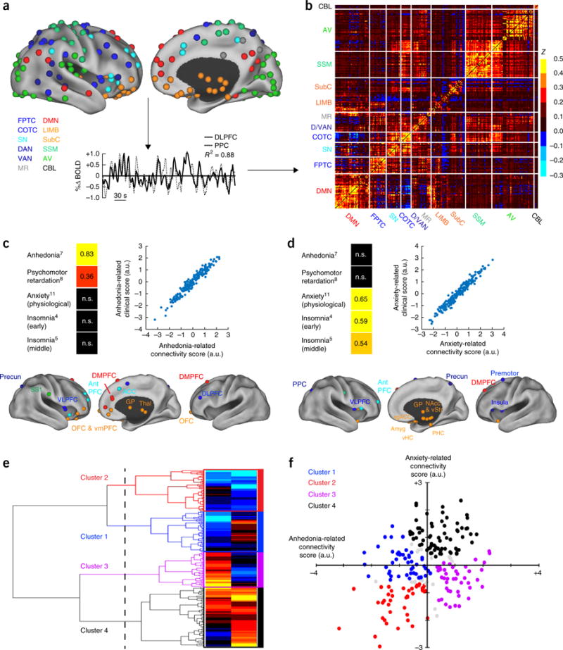
Drysdale et al., Nat. Med. 2017, Fig. 1; Dinga et al., NeuroImage: Clinical 2019

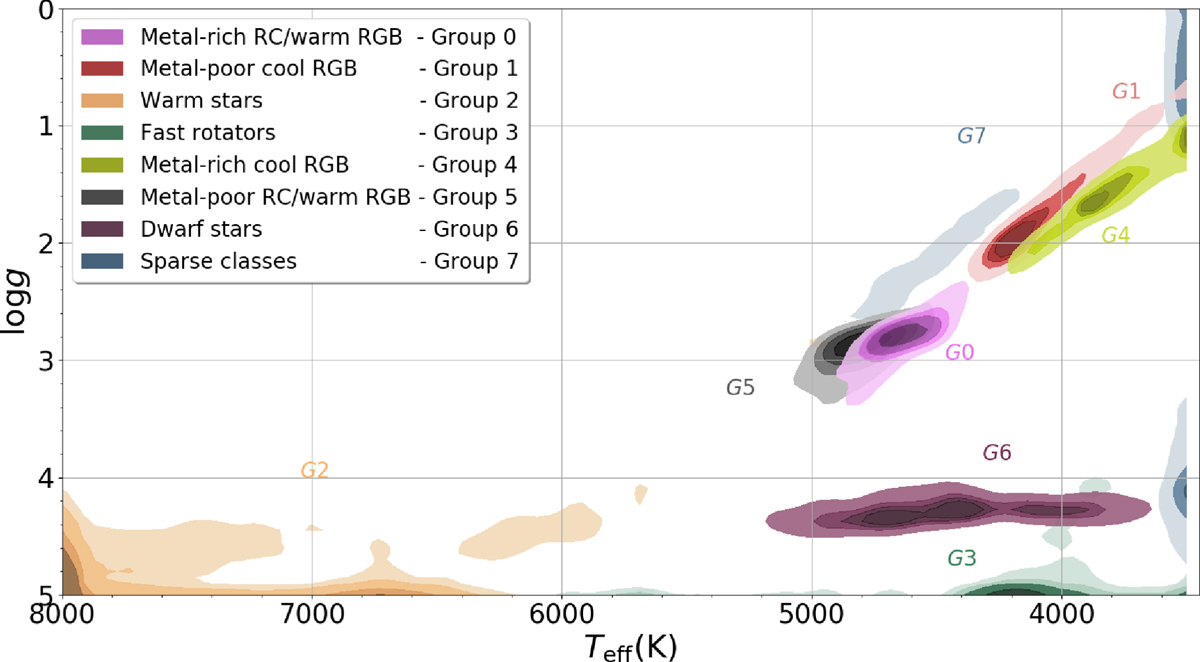
same lesson, even in physics

  • APOGEE survey. 153,847 stellar spectra. k-means in raw flux
  • some real populations recover: dwarfs vs. giants, bulge vs. halo
  • authors: “a discrete classification in flux space does not result in a neat organisation in the parameters space”
  • sensitive to initialization too
  • populations real, features wrong — flux distance ≠ physics distance

Garcia-Dias et al., Astronomy & Astrophysics 2018, Fig. 9

same lesson, four fields

  • biology — Tabula Muris: clustering as scaffolding, validated by external marker-gene priors → GOOD
  • medicine — Haldar asthma: clusters validated by RCT treatment response → GOOD
  • neuroscience — Drysdale biotypes: beautiful clusters, no permutation test, no replication → BAD
  • astrophysics — APOGEE: real populations, wrong feature space, partial recovery → MIXED

the algorithm always returns clusters. the verdict comes from what you do after the labels come out.

the clustering gotcha checklist

before reporting any cluster, ask:

  • what features did I include? — IDs, geography, dates often dominate
  • what features did I drop, and why? — feature choice is the model
  • is k defensible? — elbow + silhouette + the actual question
  • are the clusters stable?n_init=10+, multiple seeds, ARI heatmap
  • can I name each cluster from its profile? — if not, it’s an artifact
  • does the clustering answer a question someone has? — if no, don’t ship
  • what value judgment does the feature choice embed? — every feature set is a theory of similarity

summary

  • k-means — assign, recompute, repeat; minimizes SSE = \sum_k \sum_{i \in C_k} \|x_i - \mu_k\|^2
  • standardize — same lesson as PCA, Euclidean distance can’t see units
  • elbow + silhouette — rule out bad choices, not oracles for k
  • non-deterministic — different seeds, different clusters; Rand-index / ARI quantifies agreement
  • your features pick your clusters — same 317 players → archetypes, tiers, or skill ladder; feature choice scrambles partitions more than seed or algorithm
  • validate from outside — trust comes from external evidence (marker genes, RCT outcomes, replication), not from the clustering itself

next: when validation isn’t enough

we’ve trained models, tested them, validated them.

what happens when the world changes after we deploy?

  • temporal leakage — random splits leak future information
  • feedback loops — predictions change the outcomes we measure
  • Goodhart’s law — every target becomes a target

feedback

what worked? what didn’t? what’s still confusing?