Lecture 14: PCA — Dimensionality Reduction

MSE 125 — Applied Statistics

Madeleine Udell

Wednesday, May 13, 2026

logistics

• project midterm report due Friday May 15
• HW 4 out later this week — trees + PCA + clustering + Kaggle challenge

START RECORDING.

Quiz 6 covers Ch 11 (multiple testing) and Ch 13 (trees). HW 4 lands Monday and covers everything from regression inference through clustering.

Today we step out of supervised learning into our first unsupervised method: PCA. No y column. No “right answer”. The job is to find structure inside the features.

the brief

risk analyst, $5B asset manager

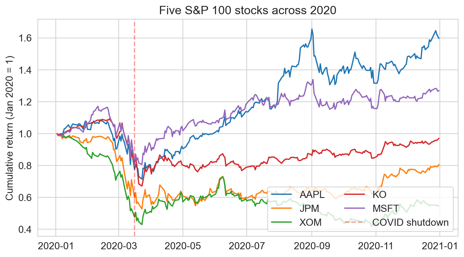
your book: S&P 100 stocks.

last March: every name crashed together

CIO asks: what risk are we really exposed to?

The decision frame: a risk analyst whose CIO wants to know what the book is exposed to. “95 stocks” is not what a CIO wants to hear — they want the systematic exposures: market beta, sector tilt, style tilt. PCA’s answer (block 2): PC1 is the market factor, PC2 is cyclicals-vs-defensives, PC3 is growth-vs-yield. Three numbers per stock, an interpretable risk decomposition for the one-pager.

The hook plot (right column) shows five S&P 100 stocks across 2020 — AAPL, JPM, XOM, KO, MSFT. For January and February the lines drift apart; mid-March they all crash together (red dashed = COVID shutdown); by summer they diverge — tech up, energy lagging. The COVID moment is the live demonstration of “every name crashed together” — sets up the question of how to summarize that risk.

Don’t spoil the punchline (PC1 explains ~40% of variance after standardization, and a 3-factor model wins on held-out portfolio variance). Hold for blocks 2 and 3.

About 1 min.

today

• the picture — geometry of the best line, then the best subspace
• reading the components — what PC1 / PC2 / PC3 mean for the S&P 100
• the payoff — minimum-variance portfolios in the p > n regime

Three blocks. Block 1 is geometry: Pearson 1901 + JPM/BAC scatter, then standardization. Block 2 is interpretation: scree plot, named factors, then the variational + SVD math. Block 3 is the practical payoff: factor-model covariance unlocks portfolios when you have more stocks than days.

The thread that runs through all three: interpretability is not validation. The named factors are appealing, but the proof PCA works comes from held-out portfolio variance, not from how nicely we can name PC2.

About 30 sec.

bridge from supervised learning

	regression / classification	PCA
input	features X + label y	features X only
goal	predict y from X	summarize X in k \ll p dims
evaluation	held-out prediction error	(today: held-out portfolio variance)
family	supervised	unsupervised

no y, no “right answer”. the algorithm finds structure on its own.

The bridge slide. Everything since Ch 4 has been supervised — there was always a y column. PCA is our first unsupervised method: no y, no labels, no “answer key”. The job is to find structure that’s already in the features.

The evaluation row is interesting — without a y, there’s no obvious held-out metric. We’ll have to invent one (held-out portfolio variance), and the chapter’s central methodological move is to use that as the validation, not the prettiness of the loadings.

K-means (next lecture) is also unsupervised; today’s PCA and Monday’s clustering are the unsupervised pair.

About 90 sec.

the picture: best line, best subspace

Pearson 1901 — same picture, drawn before computers

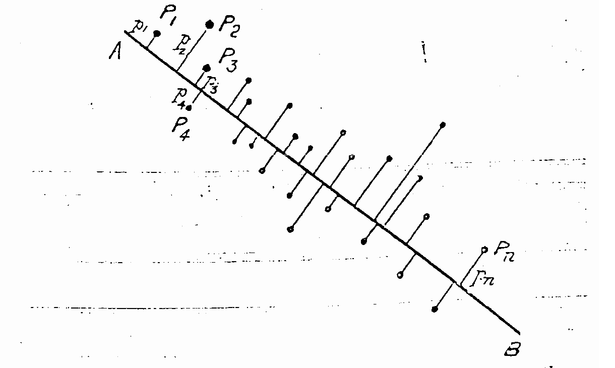
Pearson, Phil. Mag. 1901

given a cloud of points, what line minimizes the sum of squared perpendicular distances from points to the line?

Pearson answered this in any number of dimensions

— just elementary geometry

PCA is over a century old. Karl Pearson asked the question in 1901 and answered it in any number of dimensions with elementary geometry. The figure on the left is from the original Philosophical Magazine paper: a line AB through a cloud of points, with perpendicular drops p_i from each point to the line.

PCA picks the line that minimizes \sum p_i^2. That’s the whole problem. The eigenvalues and SVD come in as the answer, not the question.

Spend a moment on the figure: students will see the original from over a century ago and recognize what it shows immediately. Same problem we’ll solve today on stocks.

About 90 sec.

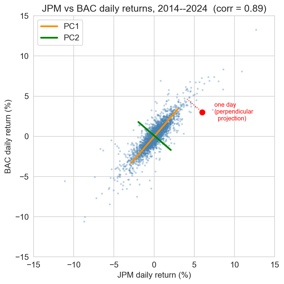
same picture, real data — JPMorgan vs Bank of America

The same Pearson picture, drawn on real data. Each blue dot is one trading day’s pair of returns: JPM on the x-axis, BAC on the y-axis, 2014–2024. Two big banks; correlation 0.89.

The cloud is elliptical. PC1 (orange) is the long axis — the shared up/down move of the two banks. Call it the “banking sector” direction. PC2 (green) is the short axis — what’s left after the common move is subtracted, the small idiosyncratic difference between the two stocks.

The dotted red line shows one day’s perpendicular drop onto PC1. Its squared length is what PCA minimizes, summed over all days.

About 2 min — let students absorb the geometry.

PC1 by hand — two stocks, a few lines

# 2x2 covariance, then top eigenvector (sorted largest first)
C = np.cov(jpm_centered, bac_centered, ddof=1)
eigvals, eigvecs = np.linalg.eigh(C)
order = np.argsort(eigvals)[::-1]
v1 = eigvecs[:, order[0]]                  # PC1 direction

# project the example day onto PC1
score = (np.array([6.0, 3.0]) - mean_xy) @ v1

PC1 direction       : (+0.653, +0.757)
PC1 variance share  : 94.4%
PC2 variance share  :  5.6%
Example day score on PC1: +6.12

The whole computation in four lines. Two banks, two PCs, no mystery.

• PC1 direction = (+0.65, +0.76) — both positive, both around 0.7. Northeast in the JPM-BAC plane. The “banking sector” direction in numbers.
• PC1 variance share = 94.4% of the total variance lives along PC1. PC2 picks up the rest.
• Example day score = +6.12. The day with JPM up 6%, BAC up 3% projects far out along PC1 — almost the whole move is sector co-movement, only a sliver is BAC-vs-JPM idiosyncratic.

Scaling to 95 stocks doesn’t change the recipe — only the size of the matrix.

About 90 sec.

scaling up — 95 stocks, same problem

returns = pd.read_csv('sp100_daily_returns_2014_2024.csv',
                      index_col=0, parse_dates=True)
print(returns.shape)

(2770, 95)

the data matrix X has shape n \times p   —   rows = 2770 days, columns = 95 stocks

now what? in 2D we drew a picture. in 95D we run the same eigendecomposition (or its rectangular cousin, the SVD — coming up).

The 95-stock dataset. 2,770 trading days × 95 surviving S&P 100 names. The 95 × 95 sample covariance has 95 eigenvalues and 95 eigenvectors — same eigendecomposition we just ran on 2×2, only larger.

We can’t draw a 95-dimensional cloud, but the math is identical: find the unit direction v \in \mathbb{R}^{95} that maximizes the variance of projected points.

About 30 sec.

predict before we run it.

we run PCA on the 95 stocks without standardizing (raw returns).

which stocks dominate PC1?

• 1. the largest companies (Apple, Microsoft, Berkshire)
• 2. the most volatile stocks (Tesla, semiconductors)
• 3. the financials (banks, insurance)
• 4. PC1 will be roughly equal across all 95

DISCUSSION: poll (2 min). Quick hands. Sets up the standardization reveal.

Target: (b) — the most volatile stocks. Without standardization, PCA finds whichever direction has the largest raw variance. Tesla swings 5% on a slow day; Coca-Cola barely moves 1%. So Tesla and the other big movers dominate PC1’s loadings.

If a student picks (a), the largest companies — that’s a natural confusion (large cap → large index weight) but PCA doesn’t see market caps, just the variance of returns. If they pick (d), they’re imagining the market factor — that’s correct after standardization but not before.

Reveal on the next slide.

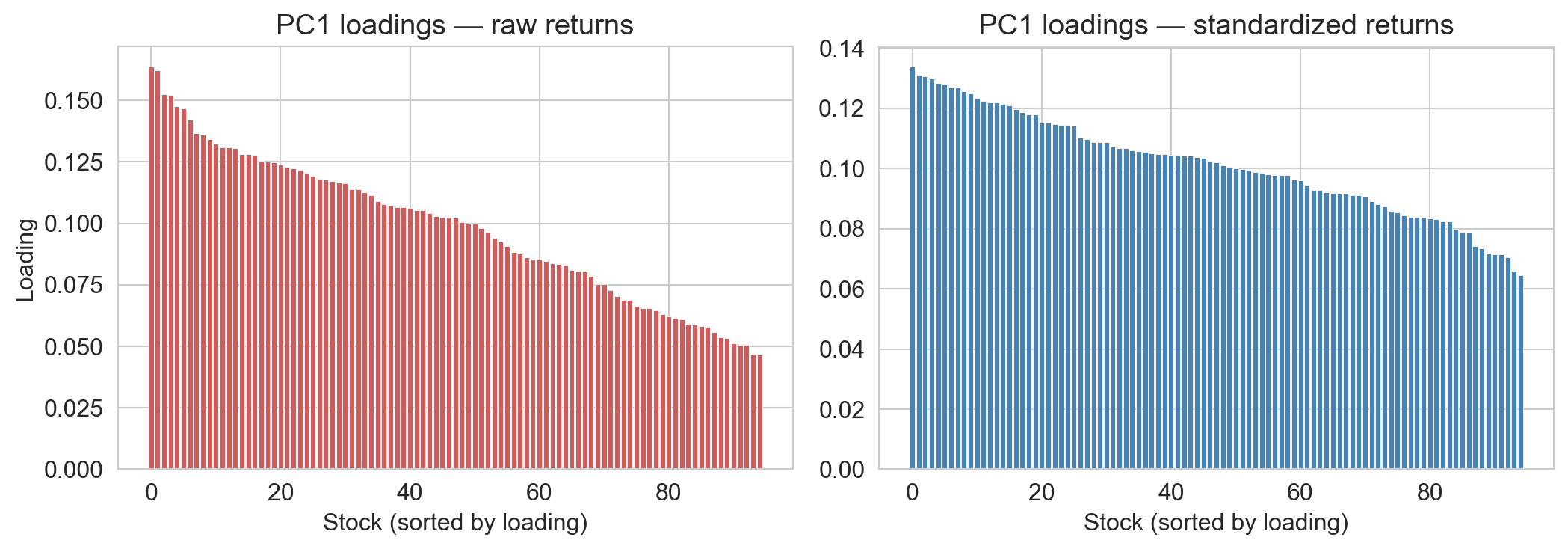
without standardization — high-vol stocks dominate

top 5 by |PC1 loading|

raw		standardized
AMD	0.164	BLK	0.134
NVDA	0.162	HON	0.131
COF	0.153	MS	0.131
TSLA	0.152	JPM	0.130
BA	0.148	C	0.128

→ raw: semis, EV, aerospace — the loud names, top 5 hold ~12%

→ standardized: financials — the most market-correlated, top 5 hold ~8.5% (baseline 5.3%)

The contrast plot. Both panels show PC1 loadings sorted from largest to smallest, but the y-axis tells the story.

Left (raw returns): steep nose, long flat tail. The top five most volatile names hold ~12% of PC1’s squared mass — more than 2× their uniform-baseline share of 5/95 ≈ 5.3%. PC1 is shaped by “TSLA and the other big movers”, not the average company.

Right (standardized): broad, uniformly positive bar. Every stock contributes nearly equally. The top-5 share drops to ~8.5%, much closer to the uniform baseline.

Same data, same algorithm — different scale.

the fix — standardize before PCA

standardization (z-score)

subtract each feature’s mean, divide by its standard deviation

z_{ij} = \frac{x_{ij} - \mu_j}{\sigma_j}

after standardization, every column has mean 0 and variance 1

→ PCA finds structure in the correlations, not the raw magnitudes

→ for returns, this is almost always what we want

The fix. StandardScaler in sklearn does this in one line. The mathematical statement: PCA on raw centered data decomposes the covariance matrix; PCA on standardized data decomposes the correlation matrix.

For returns specifically, the correlation matrix is what we want — we care about which stocks move together, not which stocks are loudest. For other problems (image processing, where every pixel is on the same 0–255 scale) standardization may not matter as much, but the rule of thumb is: standardize unless you have a reason not to.

About 60 sec.

reading the components

the scree plot — variance per PC

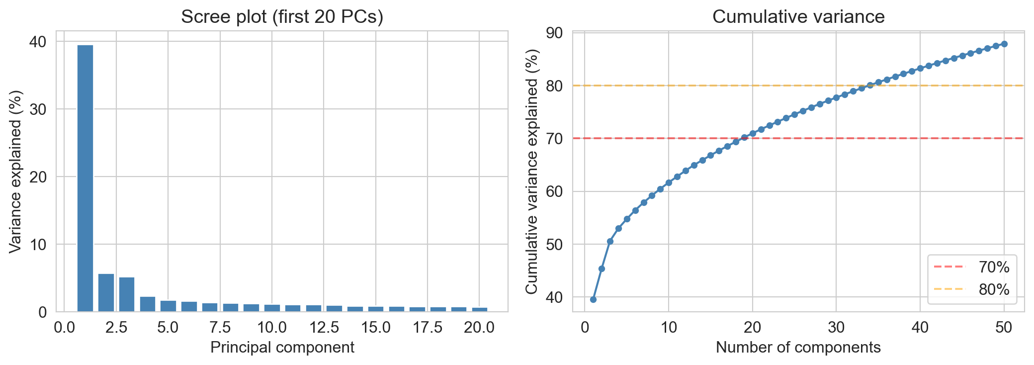
• PC1 alone: ~40% of variance
• 70% needs ~20 PCs; 80% needs ~35
• one big factor + a long flat tail — typical of equity returns

The scree plot from the chapter. Left: bar chart of variance explained by each PC. PC1 dominates at ~40%; PC2 and PC3 are small but visible (~5% each); the tail is long and gradual. Right: cumulative variance — 70% takes ~20 components, 80% takes ~35.

A naive “elbow” reading would pick k=1 — there’s a sharp drop after PC1. Hold that — we’ll see in block 3 that cross-validation actually picks k=3 instead. Different objectives, different answers.

The shape (“one big factor + long tail”) is the textbook signature of equity returns: the market factor swamps everything; sector and style factors are smaller but real; the rest is idiosyncratic.

About 90 sec.

elbow method — a heuristic, not a formula

elbow method

choose k where the scree bars stop dropping quickly — the bend in the plot

• before the elbow: meaningful structure
• after the elbow: noise

Warning

the elbow can mislead. on real data, even a sharp elbow may not pick the k that wins on a downstream task.

The elbow method is the standard heuristic. It’s a useful sanity check but not a decision rule.

The chapter’s empirical demonstration: the scree elbow says k=1, but cross-validation (block 3) picks k=3. The elbow ranks PCs by training variance — and PC1 swamps the others. CV ranks them by held-out portfolio variance — and PC2, PC3 stabilize the covariance estimate enough to matter, even though they add little to total variance.

Moral: pick k by what wins on the task you care about, not by what looks elbow-shaped on the scree.

About 60 sec.

interpret PC1 — the market factor

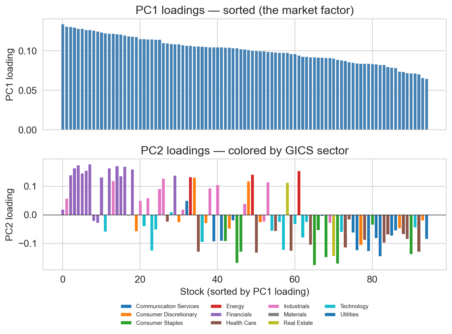
top: every stock loads positively → PC1 is the common up-down move

bottom (PC2, sectors): financials + energy on top; staples + utilities on bottom

→ PC2 = cyclicals vs defensives

The named-factor reveal. Each PC is a vector of weights, one per stock — the loadings.

Top panel (PC1): every loading is positive. A stock’s PC1 loading is its sensitivity to the market — a high-beta stock swings hard when the index swings; a defensive name has a smaller loading. PC1 is the textbook market factor.

Bottom panel (PC2, colored by GICS sector): sharp pattern by sector. Purple bars (Financials — JPM, BAC, WFC, C, COF) are positive. Red bars (Energy) also positive. Green bars (Consumer Staples — PG, KO) and dark blue bars (Utilities) are negative. PC2 is the cyclical-vs-defensive contrast — when the economy’s strong and cyclicals rally, PC2 is up; when investors flee to safety in staples and utilities, PC2 is down.

PCA discovered this without anyone telling it about sectors. The factors fell out of the eigendecomposition.

About 2 min.

interpret PC3 — growth vs yield

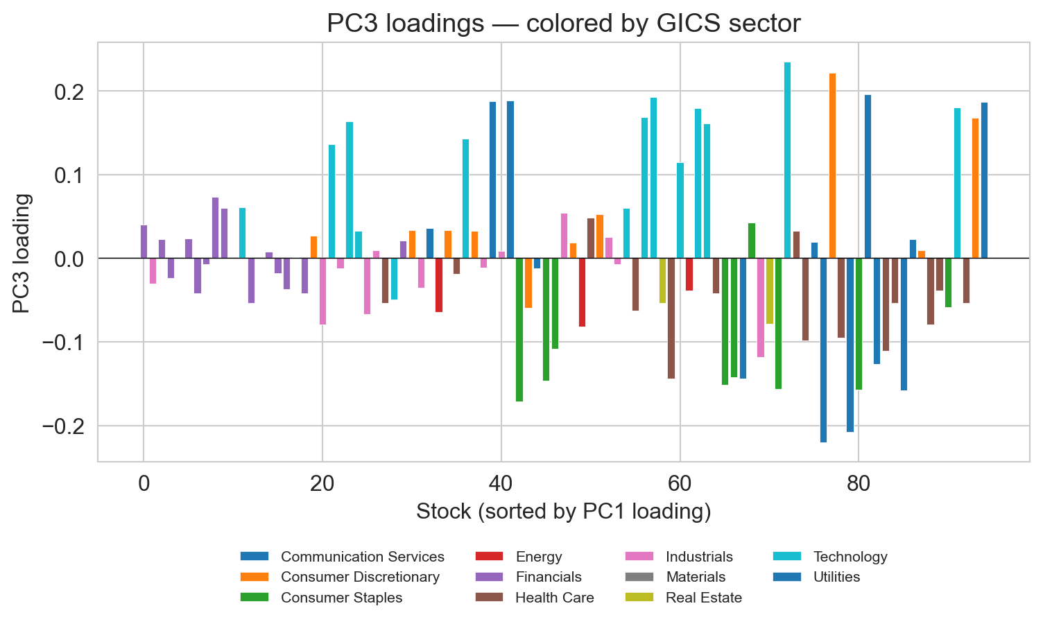
positive: NVDA, AMZN, META, GOOGL, ADBE — growth tech

negative: utilities (DUK, SO), staples (KO), high-dividend telecom (VZ) — yield

by PC5 or PC6, the economic story runs out

PC3 is the growth-versus-yield axis. Top loaders: Nvidia, Amazon, Meta, Adobe, Alphabet — all big-tech growth. Bottom loaders: utilities, staples, high-dividend telecom — the yield/income end of the market.

By PC5 or PC6 the loadings stop telling crisp economic stories — those PCs are stabilizing the covariance estimate but not corresponding to nameable factors.

About 60 sec.

we have named factors. did PCA work?

PC1 looks like the market. PC2 splits cyclicals from defensives. PC3 splits growth from yield.

have we proved PCA worked on the S&P 100?

discuss with your neighbor (3 min).

DISCUSSION: think-pair-share (3 min). 1 min think + 2 min pair. Set up the chapter’s central methodological lesson.

Target answer: no. Beautifully named factors are appealing — they pass the human-narrative test — but they’re not validation. The factors named themselves because we already know the universe: we know what financials are, we know what utilities are, so when PC2 lines up with “financials high, utilities low” we recognize the story.

What if we’d run PCA on a less-familiar dataset — gene expression, image pixels, customer behavior? We wouldn’t have the named-factor crutch. We need a method-agnostic test of whether the components carry useful information.

The chapter’s answer (block 3): use the components on a downstream task and evaluate on data we never used to fit them. Interpretability is not validation.

If a student says “yes, the named factors prove it” — that’s exactly the position the chapter argues against. Hold that and let block 3 unsettle it.

the math — what is PCA solving?

PCA (variational form)

among all k-dimensional subspaces of \mathbb{R}^p, PCA picks the one closest to the data:

S^\star = \arg\min_{\dim S = k}\; \sum_{i=1}^n \|x_i - P_S x_i\|^2

equivalently (by Pythagoras, after centering): the subspace that maximizes the total variance of the projections

with k=1: the best line through the cloud (Pearson’s picture)

with k=2: the best plane. with k general: the best k-dim subspace.

The variational form is the cleanest statement of what PCA solves. Among all k-dim subspaces of \mathbb{R}^p, pick the one minimizing total squared distance from the data.

By Pythagoras (after centering): for each point, \|x_i\|^2 = \|\text{projection}\|^2 + \|\text{residual}\|^2. So minimizing residual = maximizing projected variance. Two ways to say the same thing.

The continuity from Pearson to today: k=1 is Pearson’s line; k=2 is a plane through the cloud; for our stocks, k=3 is a 3D subspace inside \mathbb{R}^{95} — the “best” 3D summary of 95 stocks.

About 90 sec.

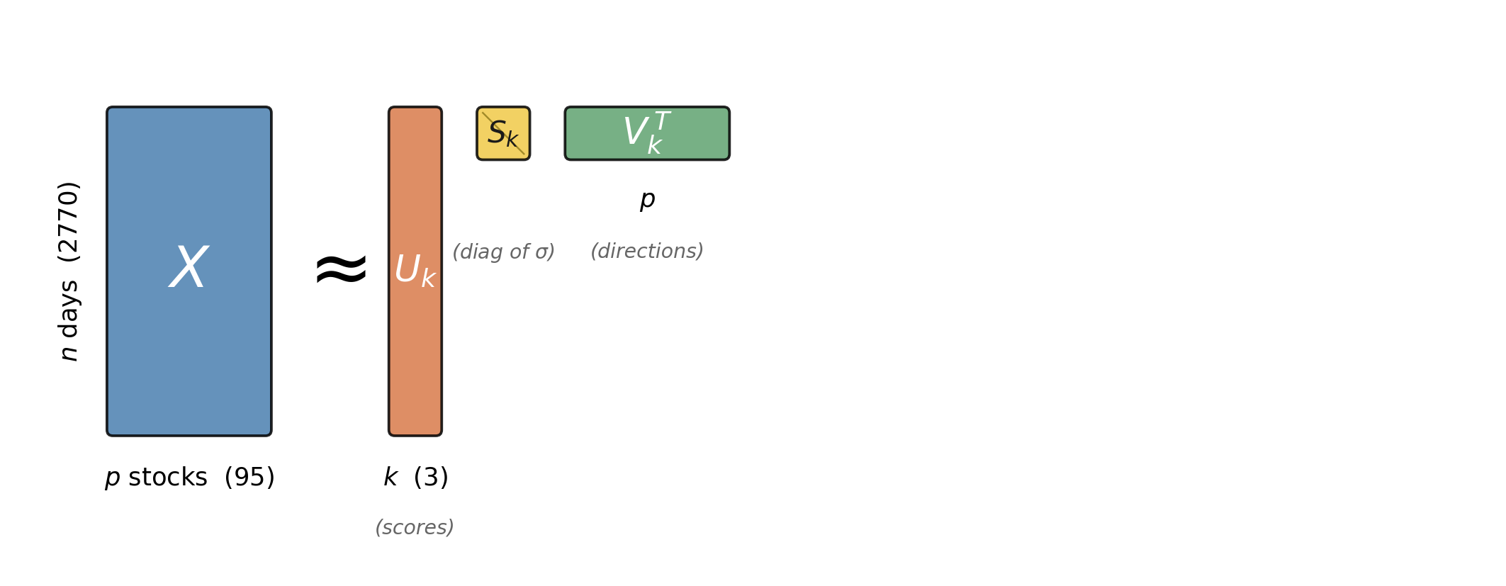
the math — how do we solve it?

data matrix X \in \mathbb{R}^{n \times p}   —   row i = x_i

• 2 stocks (earlier): eigendecomposed the 2 \times 2 covariance
• general X: truncated SVD   X \approx U_k S_k V_k^T   (works directly on X — no covariance to form)

what each piece means

symbol	size	meaning
V_k	p \times k	principal directions — basis for S^\star
U_k S_k	n \times k	projected scores — each row = one day’s coordinates
\Lambda_k = S_k^2/(n{-}1)	k \times k	PC variances

→ truncated SVD = best rank-k approximation to X in Frobenius error (Eckart–Young–Mirsky)

The variational form said what; the SVD says how. Every n \times p matrix factors as X = U S V^T with U, V orthonormal columns and S diagonal. The first k columns of V are PC1, …, PCk — the basis for the optimal subspace.

The variance of PC_i is the squared singular value over (n-1) — what sklearn returns in explained_variance_.

The cheat-sheet table at the bottom is for students who flip between sklearn docs, the finance literature, and us. Three communities, three names for the same objects. The same row in the table is the same column of V.

Don’t dwell on the table — point at it as a reference and move on.

About 90 sec.

verify — PCA() is the truncated SVD

U, S_svd, Vt_svd = np.linalg.svd(Z, full_matrices=False)

# Match up to a sign per component (sign of a PC is arbitrary)
signs = np.sign((Vt_svd[:3] * pca.components_[:3]).sum(axis=1))
print("max difference in directions:",
      np.abs(Vt_svd[:3] * signs[:, None] - pca.components_[:3]).max())
print("max difference in variances:",
      np.abs(S_svd[:3]**2 / (n-1) - pca.explained_variance_[:3]).max())

max difference in directions: 1.4e-15
max difference in variances:  3.5e-17

PCA() and np.linalg.svd give the same answer to numerical precision

A check we can run in five lines. The SVD components match sklearn’s .components_ up to a sign per PC (which is arbitrary — PC1 and -PC1 span the same line); the squared singular values divided by n-1 match the explained variances.

Differences at 10^{-15} to 10^{-17} are floating-point noise, not real. The two routines compute the same object, just packaged differently.

This is a worthwhile habit — when a textbook says “X is just Y”, verify it on a real dataset before believing it.

About 60 sec.

the payoff: portfolios in the p > n regime

why minimum variance? compounding

• two portfolios with the same average return don’t earn the same dollars
• a portfolio that loses 50% then gains 50% finishes down 25%, not flat
• compounding punishes losses more than gains

→ cutting volatility while holding return constant grows real wealth over time

→ low-volatility ETFs and pension-fund mandates: this is exactly their target

full Markowitz problem trades off return and variance; we focus on variance because that’s where covariance estimation — and PCA — bites

The motivation slide. Students will instinctively want to maximize return, not minimize variance. The honest answer is: high variance kills long-run wealth.

Walk through the 50%/50% example: $1 → $0.50 → $0.75. Down 25%, not flat. Compounding penalizes losses more than gains because the loss eats your base. The general statement: E[\log(1 + r)] \approx \mu - \sigma^2/2 — variance subtracts directly from compound growth (“volatility drag”).

Practical: low-volatility ETFs (USMV, SPLV) are billion-dollar funds. Pension funds and risk-parity strategies are explicitly variance-minimizing. So minimum-variance isn’t a quirky academic objective — it’s a major chunk of how real money actually invests.

The parenthetical at the bottom acknowledges what we’re not covering: the full Markowitz problem trades off return AND variance. We focus on the variance side because PCA is what helps us estimate covariance — and you need that to do anything else with \Sigma.

About 90 sec.

minimum-variance portfolio — Markowitz 1952

minimize portfolio variance, subject to weights summing to 1:

\min_w \, w^T \Sigma w \quad \text{s.t.} \quad \mathbf{1}^T w = 1

closed form:    w_{\text{min-var}} \propto \Sigma^{-1} \mathbf{1}

read it qualitatively:

• low-variance stocks get larger weights — less risk per dollar
• natural hedges (negative covariances) get larger weights — cancel each other
• volatile + correlated names get smaller weights — redundant risk

→ to use this, we need \Sigma — and to invert it

Markowitz, J. Finance 1952

The Markowitz minimum-variance portfolio. Two-line problem: - Variance of the portfolio’s return is w^T \Sigma w - Subject to weights summing to 1, the solution is w \propto \Sigma^{-1} \mathbf{1}

Read the inverse-row-sum interpretation: a low-variance stock with low correlations to others has a small inverse-covariance row sum dominating its row — actually it’s a bit more subtle, but the qualitative read is right: low-vol stocks and natural hedges get larger weights, volatile and correlated stocks get smaller.

So we need \Sigma^{-1}. Where do we get \Sigma? In practice, from a recent window of historical returns.

About 90 sec.

the failure mode — p > n

60-day window with 95 stocks:   p = 95,   n = 60

sample covariance is rank-deficient

59 nonzero eigenvalues out of 95 → singular → inverse doesn’t exist

even with a tiny ridge (\lambda = 10^{-6}), the “min-variance” portfolio is unusable:

max single-stock weight	+32%
min single-stock weight	−29%
gross exposure (long + short)	809%
max weight change after shifting window 1 day	9% per stock

→ not investable — we need a structured estimate of \Sigma

The crisis. We have 95 stocks but only 60 days of recent history. The 95 × 95 sample covariance from 60 observations has rank at most 59 (centering uses one degree of freedom) — it’s singular, the inverse doesn’t exist, the Markowitz formula crashes.

Adding a small ridge (\Sigma + \lambda I) makes it invertible but not stable: weights become enormous, change wildly with a one-day shift in the estimation window. Useless in practice.

The math we were taught for \Sigma^{-1} assumed n \gg p. In high-dim finance, that’s rarely true. We need a structured estimate of \Sigma.

About 60 sec.

PCA gives us \Sigma — the factor model

approximate \Sigma as k factors + diagonal noise:

\hat\Sigma_k = V_k \Lambda_k V_k^T + \mathrm{diag}(D)

• V_k = top k PC directions (the factors)
• \Lambda_k = diagonal of PC variances
• \mathrm{diag}(D) = stock-specific residual — ensures \mathrm{diag}(\hat\Sigma_k) = 1 on standardized data

→ \hat\Sigma_k^{-1} exists, plugs cleanly into Markowitz

→ how big should k be? ask cross-validation

The fix. Instead of estimating the full 95 \times 95 covariance from 60 days, we constrain it: assume the structure is k pervasive factors + idiosyncratic noise.

The factor part V_k \Lambda_k V_k^T captures the systematic risk that PCA found (market, sectors, etc.). The diagonal D accounts for stock-specific risk that the factors don’t explain — and it’s what makes the estimate positive definite (so the inverse exists).

Now we have \hat\Sigma_k with rank up to \min(p, k + p) = p — invertible by construction.

The catch: we have to pick k. The scree elbow says k=1. Cross-validation will say k=3. Coming up.

About 90 sec.

the four estimators

method	formula	role
equal-weight	w = \mathbf{1}/p	baseline (no covariance)
ridge sample	\Sigma + \lambda I	invertibility hack
random projection	random V_k + diag correction	sanity check
PCA factor	top-k PC factors + diag correction	the contender

we backtest with walk-forward evaluation — train on the past, hold for the next 21 days, slide

The four estimators we’ll compare. The first two are the standard competitors any new estimator has to beat. The third — random projection — tests whether PCA’s variance-aligned directions actually matter, or whether any low-rank approximation would do. If random does as well as PCA, then the “structure” PCA finds is illusory.

The walk-forward evaluation: train on the first 60 days, hold for the next 21 (about a month between rebalances), then slide the window forward and repeat. Time-respecting CV — never train on data that comes after the test window. We’ll come back to walk-forward properly in Ch 16.

Why walk-forward instead of random 5-fold? Returns are correlated across time (volatility clusters, market regimes persist). A random fold puts March 15 in training and March 14, 16 in validation — same regime, leaks information. Random-fold validation underestimates true generalization error.

About 90 sec.

the result — variance vs k

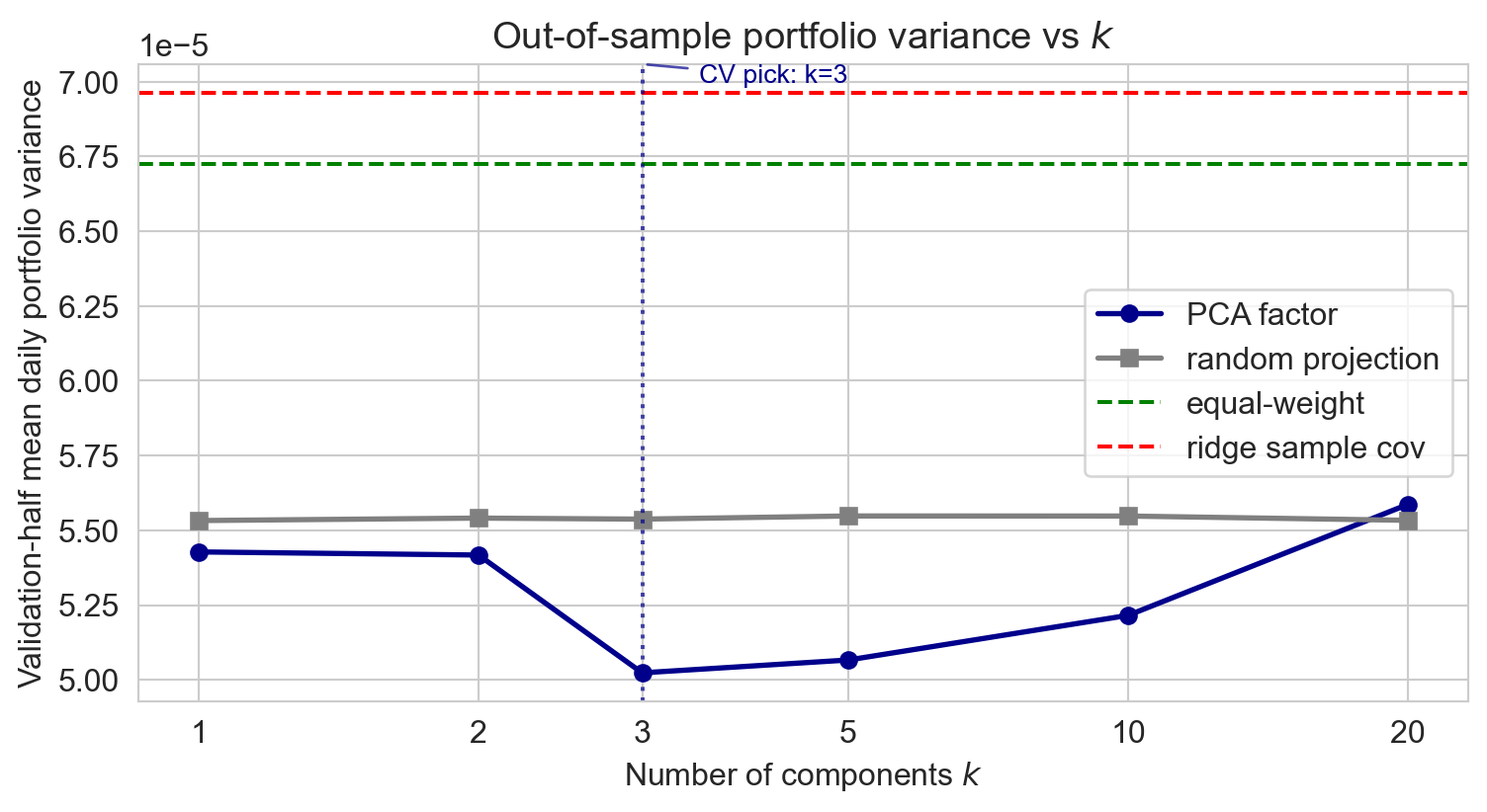
• PCA factor (blue) drops fast 1→3, flat-ish 3→10, rises past 10
• CV picks k = 3 — well below scree’s “elbow at 1”
• random projection (gray) lies above PCA throughout — variance-aligned directions matter

The CV plot. Validation-half mean daily portfolio variance vs. number of components k, log-scale on k.

Blue (PCA factor): drops sharply from k=1 to k=3 as PC2 and PC3 stabilize the covariance estimate. Flat between k=3 and k=10. Rises past k=10 as we start fitting noise — same bias-variance trade-off as in regression, but for covariance estimation.

Gray (random projection): consistently above PCA. A random low-rank approximation captures some of the structure, but always less than PCA’s variance-aligned directions. So PCA is finding signal, not just any low-rank summary.

Red dashed (ridge): worst of all. The ridge estimate is so unstable that even at any k, PCA wins by a wide margin.

Green dashed (equal-weight): beats ridge but lags PCA. Equal-weight is a tough baseline — it’s parameter-free and robust.

The CV pick is k=3. Three factors is enough to capture the systematic structure; more components start adding noise.

About 2 min.

the result — cumulative variance over time

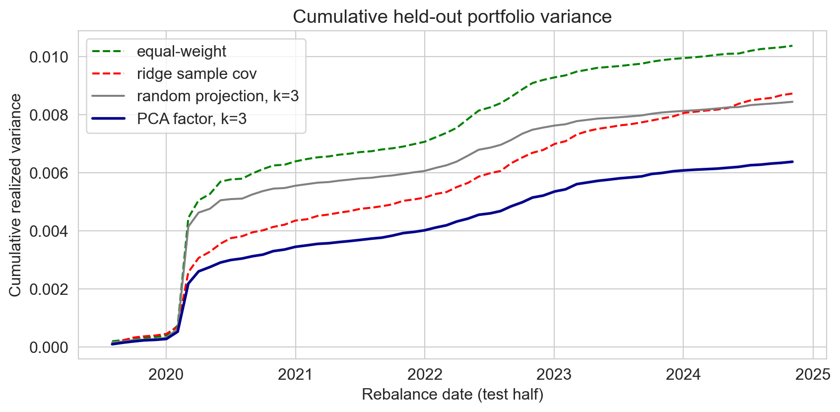
PCA factor portfolio sits lowest the entire test period

every method jumps at COVID; PCA’s jump is smallest

The cumulative-variance curves on the held-out half. Lower = better.

PCA factor (dark blue): flattest curve. Lowest cumulative realized variance from start to finish.

Ridge sample cov (red dashed): second best in this run. Still well above PCA.

Random projection (gray): captures some structure, lags PCA throughout.

Equal-weight (green): worst here, but only marginally — equal-weight is a hard baseline to beat with this much instability in the sample covariance.

The COVID jump in early 2020: every line shoots up — every covariance estimator was caught off guard, every portfolio took a variance shock. But PCA’s shock was the smallest of the four. The market’s structure changed fast in March 2020, and a factor-model estimate adapted faster than the alternatives.

About 90 sec.

interpretability is not validation

PC1 = market,   PC2 = cyclicals / defensives,   PC3 = growth / yield

→ a clean story. but a story is not the test.

the test:   held-out portfolio variance, on data we never used to fit

→ pick the model that wins on the task you care about

The chapter’s central methodological lesson, and the answer to the block-2 discussion. The named factors looked impressive, but a named factor is just a story — it doesn’t prove the method works.

The proof comes from a downstream task evaluated on data we never used to fit the components. That’s what cross-validation does for predictive models, and that’s what walk-forward backtesting does here for covariance estimation.

This is the eval-by-downstream-task rule. It’s the same idea as cross-validation in regression: don’t trust how well a model fits the training data; trust how well it predicts data you set aside.

About 60 sec.

cautionary tale — genes mirror geography

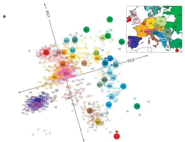
197K SNPs, 1,387 Europeans

no geographic info given to the algorithm

→ it drew a map of Europe   (r^2 \approx 0.7)

. . .

→ math result: PCA on spatial data with distance-decaying similarity generically produces these patterns

→ recovering an obvious pattern is not evidence of hidden structure

Novembre 2008; Novembre & Stephens 2008

The cautionary callout from the chapter. Novembre et al. ran PCA on ~197K SNPs across 1,387 Europeans, gave the algorithm zero geographic information, and the first two principal components — when plotted against each other — reproduced the map of Europe with high fidelity. PC1 lined up with latitude, PC2 with longitude.

The temptation is to read this as “PCA discovered hidden European population structure.” The same research community published the math showing otherwise: Novembre & Stephens (2008, Nature Genetics) proved that PCA on any spatial data with distance-decaying similarity will produce gradient/sinusoidal patterns generically — no historical demographic event required.

So the famous figure was always going to come out — the math made it inevitable given the sampling. The structure was built into the input geography, not discovered as European prehistory.

The lesson — and a parallel to today’s named-factor discussion: a PCA figure that reproduces something obvious about the data (a map, a known taxonomy) is not by itself evidence that PCA discovered hidden structure. Same lesson next lecture, on clustering. Genes mirror geography → PredPol mirrors policing → MBTI mirrors cutpoints. Three fields, same artifact.

About 2 min.

PCA or pick five?

instead of computing principal components, could we just pick the five best stocks and form a portfolio from them?

when would PCA be the right move? when would a sparse subset (Lasso) be the right move?

discuss with your neighbor (3 min).

DISCUSSION: think-pair-share (3 min). 1 min think + 2 min pair + brief debrief.

Target answers:

Lasso is the right move when the truth really is sparse — only a handful of stocks matter for predicting some outcome, the rest are noise. Example: “predict next-quarter earnings from one of 200 specific accounting ratios.” You want a short list.

PCA is the right move when many features carry useful information and you want a low-dimensional summary that pools them. Example: today’s covariance matrix where every stock is partly driven by a common market factor. A sparse subset would miss the market hitting all of them.

The third option — sparse PCA — splits the difference: principal components in which most loadings are zero. Less common, but it exists.

The deeper point: PCA and Lasso answer different questions. Lasso says “which features matter?” PCA says “what’s a low-dim summary?” Both are valid; pick by what your downstream task needs.

demo: PCA in the notebook

colab.research.google.com/…/lec14-pca.ipynb

what to watch:

• toggle standardization on/off — watch PC1 flip from “TSLA-dominated” to “market”
• vary k from 1 to 20 — watch held-out variance drop, flatten, rise
• swap in your own time window — does CV’s pick of k change?

Demo slide. The notebook has the full pipeline (standardization toggle, scree plot, factor model, walk-forward backtest); the three knobs above are the experiments worth running.

If running short: skip the live demo, point at it as homework prep. HW 4 has students do exactly this on Airbnb data.

About 30 sec.

summary

• PCA finds the directions of maximum variance — best line, best plane, best k-dim subspace
• standardize first — otherwise the largest-magnitude features dominate
• PC1, PC2, PC3 on the S&P 100 are the market, cyclical-vs-defensive, growth-vs-yield
• truncated SVD is what PCA computes (Eckart–Young–Mirsky: best rank-k approximation)
• factor-model covariance \hat\Sigma_k = V_k \Lambda_k V_k^T + \text{diag} unlocks portfolios when p > n
• interpretability is not validation — pick k by held-out task, not the scree elbow

Six takeaways, in lecture order.

The last bullet is the headline. If a student takes one thing from the lecture, it’s this: pretty loadings tell a story, but the story isn’t the test. The test is what wins on a downstream task evaluated on data you didn’t fit.

About 60 sec.

next: clustering — same template, different constraint

PCA compresses each row into continuous coordinates in a k-dim subspace

K-means compresses each row into one of k discrete labels

same compress-into-k idea, different geometry

→ Monday: K-means on Airbnb (and the same “your features pick your structure” lesson, on a different method)

Forward pointer to lec15. PCA today gives every row continuous PC scores in a low-dimensional subspace. K-means Monday will give every row a single discrete cluster label.

Mathematically these are cousins — both can be framed as low-rank approximation problems. PCA uses continuous coordinates; K-means uses one-hot indicators (each row gets weight 1 on one cluster, 0 on the rest). Same compress-into-k template.

A natural starting move on Monday: cluster the PC scores from today’s analysis rather than the raw features.

The “your features pick your structure” lesson reappears: the Novembre cautionary tale today, the PredPol cautionary tale Monday — same lesson on adjacent methods.

About 45 sec.

feedback

forms.gle/feedback

what worked? what didn’t? what’s still confusing?

Standard feedback slide. Same form as previous lectures.