Lecture 13: Decision Trees and Random Forests

MSE 125 — Applied Statistics

Madeleine Udell

Monday, May 11, 2026

logistics

• HW 3 review sessions this week
• Quiz 6 Wednesday May 13 — regression inference + trees
• project midterm report due Friday May 15

START RECORDING.

HW 3 was due Friday — graded back this week. Quiz 6 covers trees (today) and dimensionality reduction (Wednesday). Project midterm report due Friday.

the brief

Airbnb host, NYC

goal: develop a pricing tool to help hosts set competitive nightly rates

ch 5: a reasonable R^2 — but you picked the interactions, polynomial degree, and neighborhood encodings by hand

keep hand-engineering, or use a model that splits on its own?

The decision frame: a host-facing pricing tool, deadline Friday. Ch 5’s regression required hand-picking interactions, polynomial terms, and neighborhood encodings. Today we ask whether a tree-based model can find that structure on its own — and whether it’s good enough to ship.

The image (the depth-3 tree on Airbnb) is just visual furniture for now — they’ll see it in detail in block 1. Don’t decode it on this slide.

The chapter’s surprise lands in block 3: 100 averaged overfit trees beat the hand-engineered linear model.

today

• decision trees — splits found automatically, no encoding needed
• a single tree overfits — and CV picks the depth
• random forests — average overfit trees, watch variance collapse
• trees vs. linear — geometry of the data picks the model
• feature importance — what the forest uses, what to doubt

Five beats. Each block has its own discussion. Block 1 establishes how a tree splits and overfits. Block 2 introduces bagging + the surprise that 100 overfit trees beat a hand-crafted linear model. Block 3 closes with how to read (and doubt) feature importance.

bridge from logistic regression

	logistic regression	decision tree
boundary	one hyperplane	many axis-aligned cuts
feature engineering	manual (Ch 5)	automatic
categories, missing	encode + impute	native
output	probability via \sigma(\beta^\top x)	mean of leaf

both follow the same recipe: fit, score, CV, predict.

The bridge slide. Logistic and tree share the same model-fitting recipe (fit, score, CV, predict) — they differ in how they carve up the feature space. Logistic draws one hyperplane; a tree stacks axis-aligned cuts. Both use the validation tools from Ch 6 and the classifier metrics from Ch 7.

This sets up the “trees vs. linear” comparison in block 2.

how a tree splits

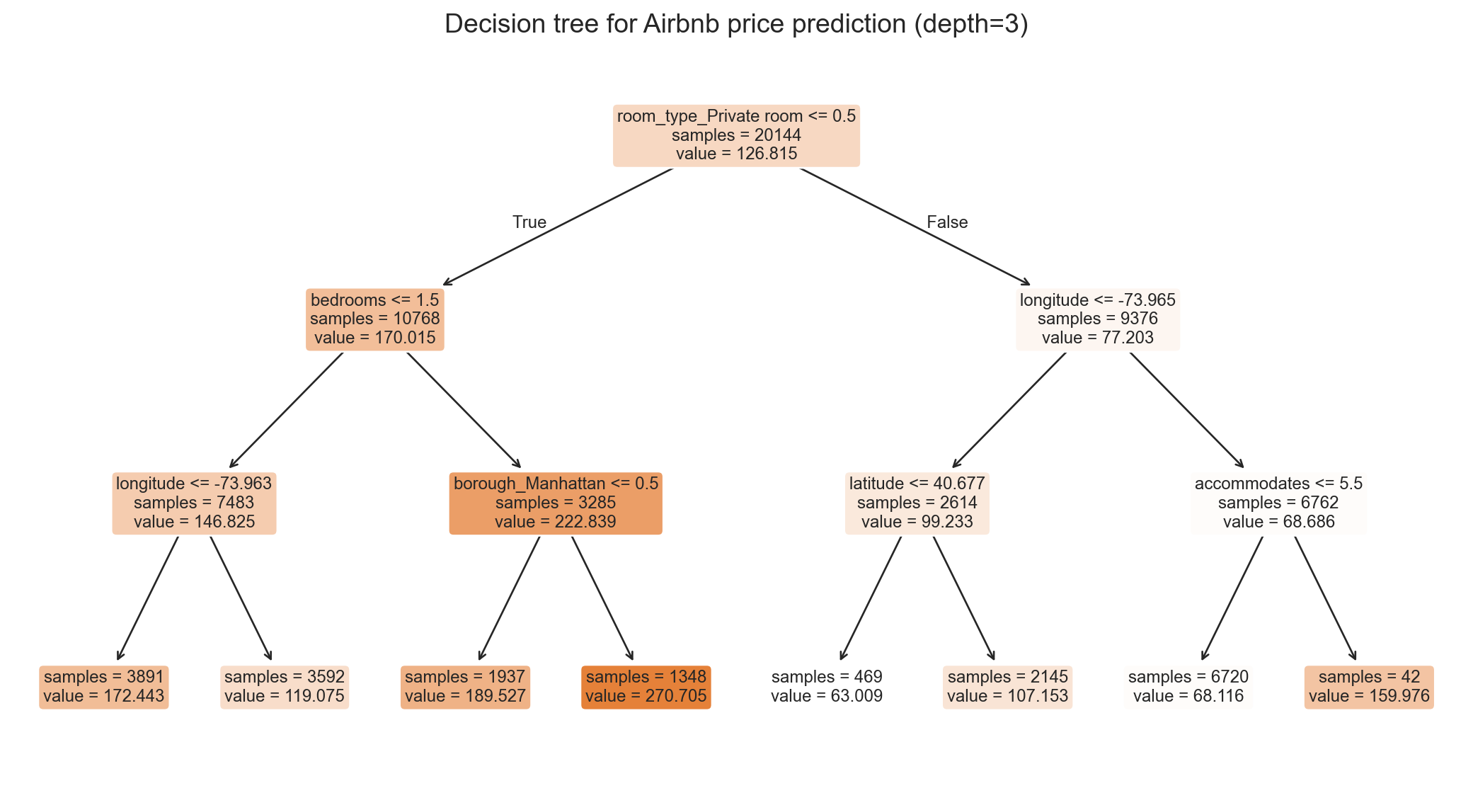
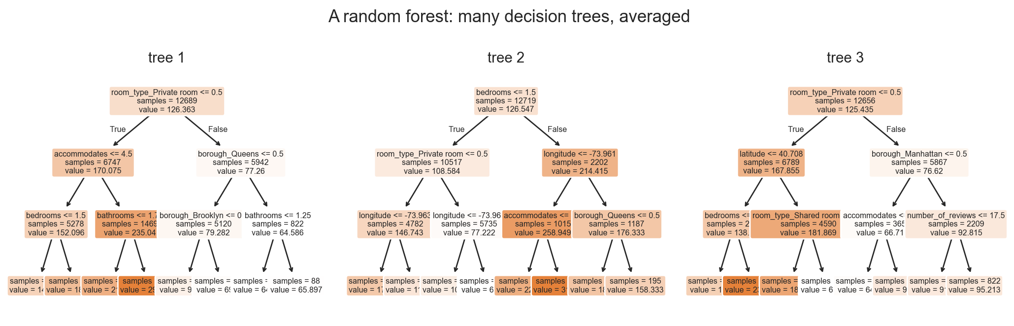
decision tree, in pictures

each leaf reports a predicted price + sample count

The depth-3 tree on Airbnb. Read top-down: each internal node asks an if/then question on one feature; each leaf is a region of feature space with a predicted price + sample count.

Don’t memorize the tree — point at the structure: room type at the root, then borough/bedrooms beneath. The model discovered these splits without any encoding hint.

About 60 sec.

tree vocabulary

decision tree

recursive if/then splits on one feature at a time

• leaf — node with no children; carries a prediction
• internal node — any non-leaf node; asks a yes/no question, routes to a child
• root — the single internal node at the top
• depth — longest root-to-leaf path
• max_depth — sklearn knob that limits depth

Definition box + vocabulary list on the left, the depth-3 tree on the right so students can pin each term to a node as they read it. Leaves = the bottom row of small boxes (no children, carry the prediction); internal nodes = every other box including the root; root = the one at the top; depth = 3 here.

If anyone asks: the root counts as an internal node (the one at the top, with no parent).

About 90 sec.

look at the second split

on the more-expensive side, the tree splits on bedrooms ≤ 1.5.

why did the algorithm pick bedrooms here, instead of bathrooms or accommodates?

INLINE PREDICT (45 sec). Reasoning prompt — students already saw the answer on slide 7, so we shift from prediction to why.

Target answer: at this node the algorithm searches every (feature, threshold) pair and picks the one that drops SSE the most. bedrooms wins because the price gap between studios/1-bedrooms and 2+ bedrooms is sharper here than the gap induced by bathroom count or accommodates count. Bathrooms and accommodates correlate with bedrooms, so they carry similar information but split less cleanly at this node.

Lesson: greedy splitting picks the most discriminating cut at this node — not the feature that’s “most important” overall. Importance is a summary, splits are local.

Quick activity, no debrief beyond a sentence.

how a split is chosen

at each node, search every (j, s) — feature j, threshold s:

\min_{j,\, s} \left[ \sum_{x_i \in R_1(j,s)} (y_i - \bar{y}_1)^2 + \sum_{x_i \in R_2(j,s)} (y_i - \bar{y}_2)^2 \right]

(sum of squared errors, SSE)

• each child predicts the mean \bar{y} of its training rows
• algorithm enumerates every (feature, threshold) pair
• pick the split that drops total SSE most
• recurse inside each child

The formal split criterion. Squared-error loss for regression: pick the (feature, threshold) pair that minimizes total within-region squared error after the split. Each leaf predicts the within-leaf mean.

Don’t dwell on the formula — students recognize SSE from Ch 4. The sketch on the next slide makes “greedy axis-aligned partitioning” concrete.

About 90 sec.

greedy partitioning, step by step

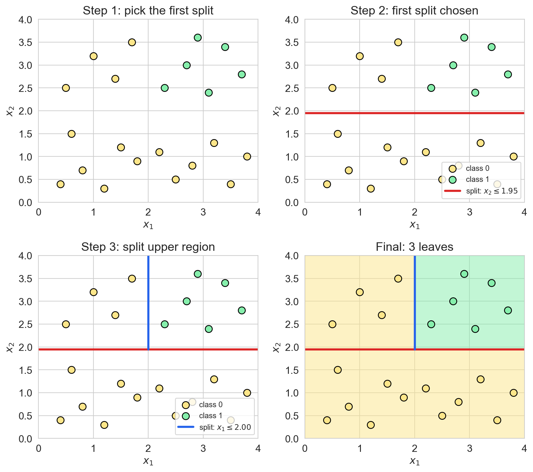
• greedy — best split now, never reconsidered
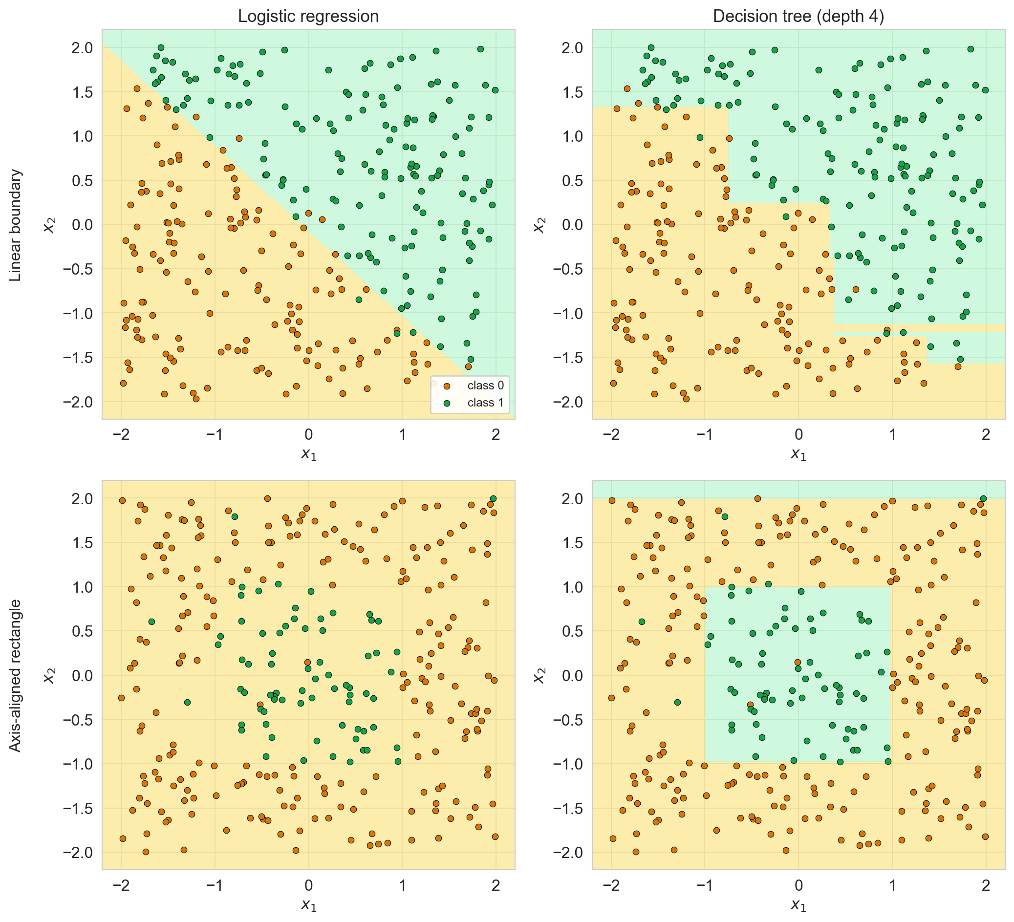
• axis-aligned — every cut parallel to an axis; a diagonal becomes a staircase

The 4-panel toy: 22 points, two classes (yellow + green), depth-2 tree. Step 1 — pick the first split. Step 2 — split on x_2 \leq 1.95 (peels off the bottom strip). Step 3 — the upper region still mixes classes; split on x_1 \leq 2.00. Final — three pure leaves.

Two takeaways below the figure: 1. Greedy: best split right now, never reconsiders. Standard practice; not guaranteed optimal (NP-hard in general). 2. Axis-aligned: every cut parallel to an axis. A diagonal boundary becomes a staircase. Comes back in block 2 (trees vs. linear).

About 2 min.

classification: same recipe, swap the loss

Gini impurity

\text{Gini} = 1 - \sum_{k=1}^K \hat p_k^2

binary case: 2\hat p (1 - \hat p)

• pure node: Gini = 0
• 50/50 binary node: Gini = 0.5
• everything else — depth, CV, evaluation — is identical

Drop the 60-second classification aside in. The only thing that changes between regression trees and classification trees is the splitting criterion: SSE becomes Gini impurity. Same greedy recursive partitioning, same depth control, same CV recipe.

Pure node = 0; perfectly mixed binary node = 0.5. Tree picks the split that drops \text{Gini}_\text{parent} - p_L \cdot \text{Gini}_L - p_R \cdot \text{Gini}_R the most — categorical analogue of “drop SSE the most.”

Don’t dwell. Block 1’s main act is what happens when you let the tree go too deep.

deep enough to memorize, shallow enough to generalize

do deep trees overfit?

we’re about to fit a single tree at depths 1–20 on Airbnb, with min_samples_leaf=5.

sketch what train R^2 and test R^2 look like as depth grows.

at what depth does test R^2 peak?

INLINE PREDICT (45 sec). Students sketch on paper. Most will know train R² rises monotonically; the prompt forces them to commit on test. Common predictions: “U-curve, peak around depth 5–7.”

Reveal on the next slide. The actual peak is at depth 7 (test R² = 0.615). That makes a clean lead-in to CV.

a single tree overfits

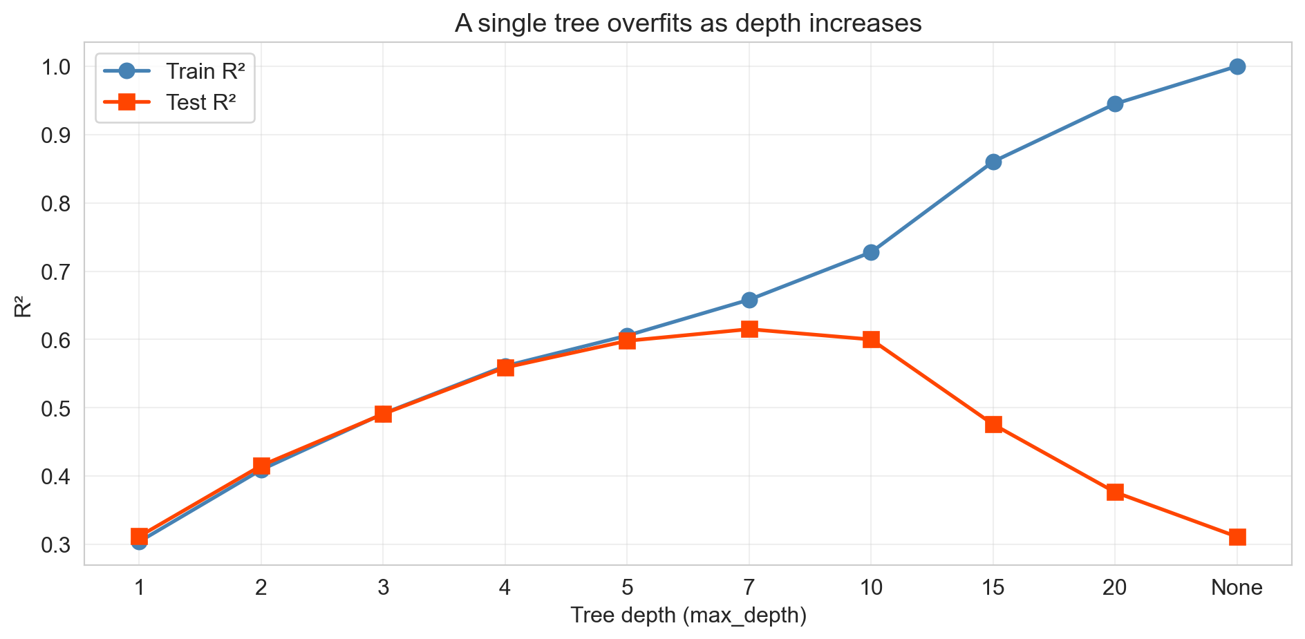
• shallow — underfits, high bias
• deep — memorizes training rows, high variance
• test R^2 peaks near depth 7, then collapses

The U-curve reveal. Train R² climbs toward 1.0 as the tree memorizes; test R² peaks near depth 7 (CV agrees on the next slide), then collapses.

Numbers worth quoting: at depth 4, train = 0.561, test = 0.559 (no overfit yet). At depth 20, train = 0.945, test = 0.376. Unrestricted, train = 1.0 (every row in its own leaf), test = 0.311.

This is the bias-variance tradeoff from Ch 6 — same shape, new “complexity knob” (max_depth instead of polynomial degree).

shallow vs. deep, on a 2D slice

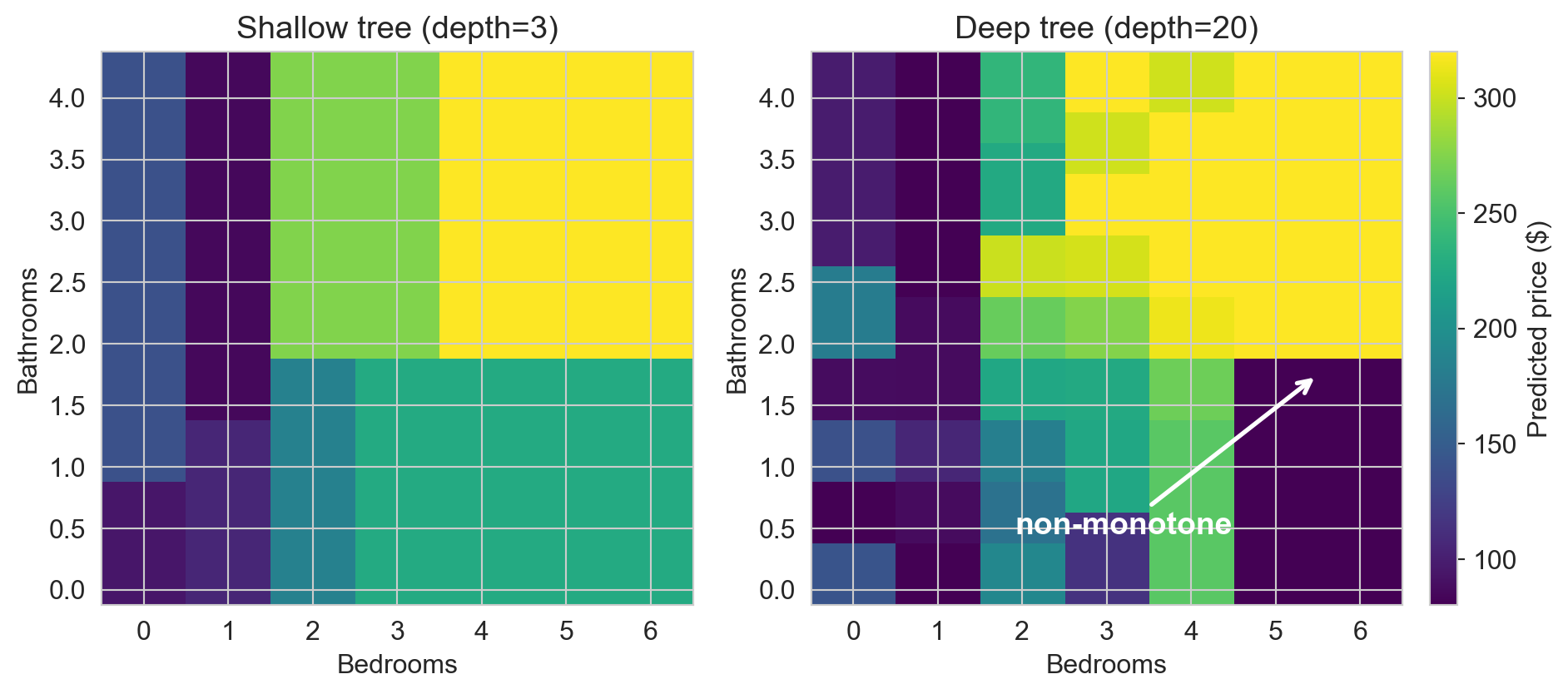
deep tree’s quilt shows memorization — adding a bedroom can lower the prediction

Two trees, both trained on (bedrooms, bathrooms) only, predicted price as color. Shallow (depth 3): a few orderly blocks — bigger listings cost more, every step. Deep (depth 20): a quilt where some adjacent cells have lower prices for more bedrooms. That non-monotone behavior means the tree has memorized a few quirky training rows.

A linear model would render the same plot as a smooth color gradient — no quilt. Trees draw rectangular blocks; that’s their signature.

CV picks the depth

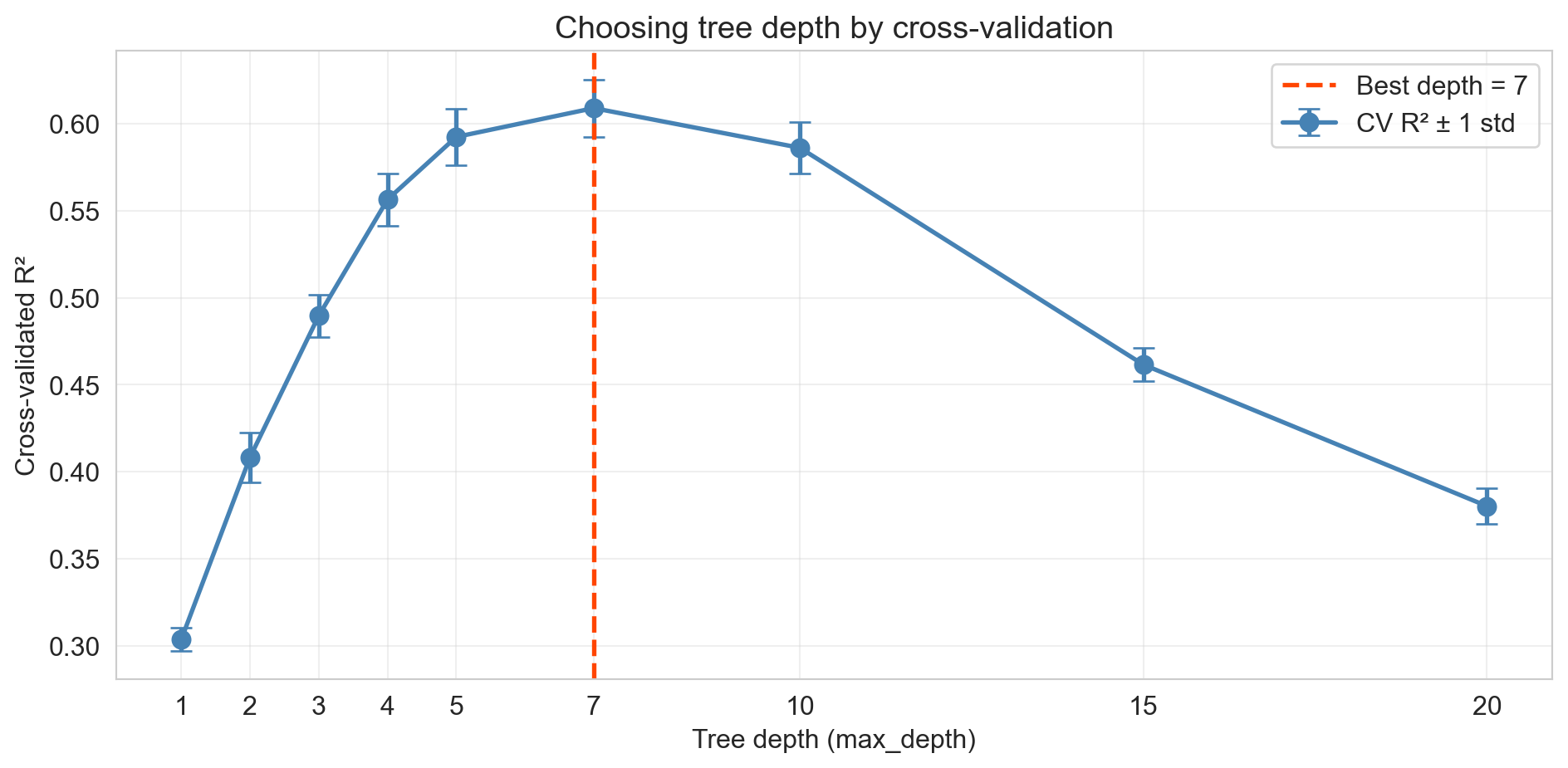
same recipe used for lasso \alpha, polynomial degree, k in kNN

The U-curve again — this time with 5-fold CV (errorbars are CV std). Best depth: 7. Test R² at the chosen depth: 0.615.

Why CV not test? Picking depth on the test set burns it for honest evaluation. CV does the tuning on training data, so the test set stays clean for a final report.

The recipe (sweep candidates, score with CV, take the best) generalizes — same thing for lasso α, polynomial degree, k in kNN, n_neighbors, anything tunable.

from regression to classification: fill in the blanks

the regression recipe: split on SSE, predict the mean \bar y.

for classification, two things change:

1. splitting criterion: SSE → ?
2. leaf prediction: mean of y → ?

INLINE PREDICT (45 sec). Two fill-in-the-blanks — conceptual, no code on screen.

1. Gini impurity (defined two slides ago). The classification splitting criterion. Same recipe — pick the split that drops Gini the most.
2. Majority class (for hard predictions) or class proportions (for soft predictions / probabilities — needed for AUC).

Everything else — depth control, CV, train/test split — stays the same. That’s the punchline: the recipe is shared; only the loss and the leaf statistic change.

If anyone asks about the performance metric: R² doesn’t apply to 0/1 outcomes; we use accuracy or AUC. That’s an evaluation choice, separate from the splitting criterion.

Quick reveal — no debrief beyond the wrap.

a host with a 20-bedroom Manhattan apartment wants a price.

both models were fit on Airbnb listings, prices in $10–$500/night.

linear regression (simplified, Manhattan, entire home): \widehat{\text{price}} = \$80 \;+\; \$30 \cdot \text{bedrooms}

depth-3 tree (Manhattan, entire home, bedrooms branch):

• bedrooms \leq 1.5 → \$135
• 1.5 < bedrooms \leq 2.5 → \$190
• bedrooms > 2.5 → \$270

1. what does each model predict for 20 bedrooms?

2. which would you trust — and why might both be wrong?

DISCUSSION: think-pair-share (5 min). 1 min think + 2 min pair + 2 min debrief.

Numerical answers (push for these first):

• Linear: 80 + 30 \cdot 20 = \$680 — the slope keeps going.
• Tree: the bedrooms > 2.5 leaf, $270 — the prediction flatlines because the tree was never trained on anything bigger.

Pedagogical points:

1. Linear extrapolates. It extends the fitted slope past the training range. If the true relationship really is linear out to 20 bedrooms, the extrapolation is roughly right; if it bends (luxury surcharges, capacity caps), it’s wrong in a smooth direction.
2. Trees flatline. A tree’s prediction is the mean training y inside one leaf. For inputs past the training range, the input routes into the boundary leaf — whose mean was calibrated on 3-, 4-, 5-bedroom listings. The tree is guaranteed to be wrong out there, by construction.
3. Both are wrong here. Training data was capped at $500; a real Manhattan 20-bedroom listing might be $5,000+. Neither model has any signal that far out.

Connects forward to the “when to doubt the forest” section: distribution shift is a forest’s weakness, not a linear-model strength.

If students get stuck on (2), prompt: “where does the training data end? what happens past that point in each model?”

average overfit trees

the random forest, briefly

random forest

ensemble of deep trees, each trained on a bootstrap sample of rows, considering only a random subset of features at each split. predictions are averaged (regression) or voted (classification).

• bagging — each tree sees different rows
• feature subsampling — each split considers different features
• trees memorize different noise → averaging shrinks variance

Direct definition. Two sources of randomness combine: bootstrap rows (Ch 8 callback) and feature subsampling. The result is an ensemble of overfit-but-different trees whose average has dramatically lower variance than any individual tree.

Image: three trees from a tiny forest (n_estimators=3, depth=3, max_features=0.3). Same top-level idea (each tree partitions the feature space), but different splits at every level — that’s the diversity averaging needs.

The next slide makes “bootstrap sample” concrete.

bootstrap samples in pictures

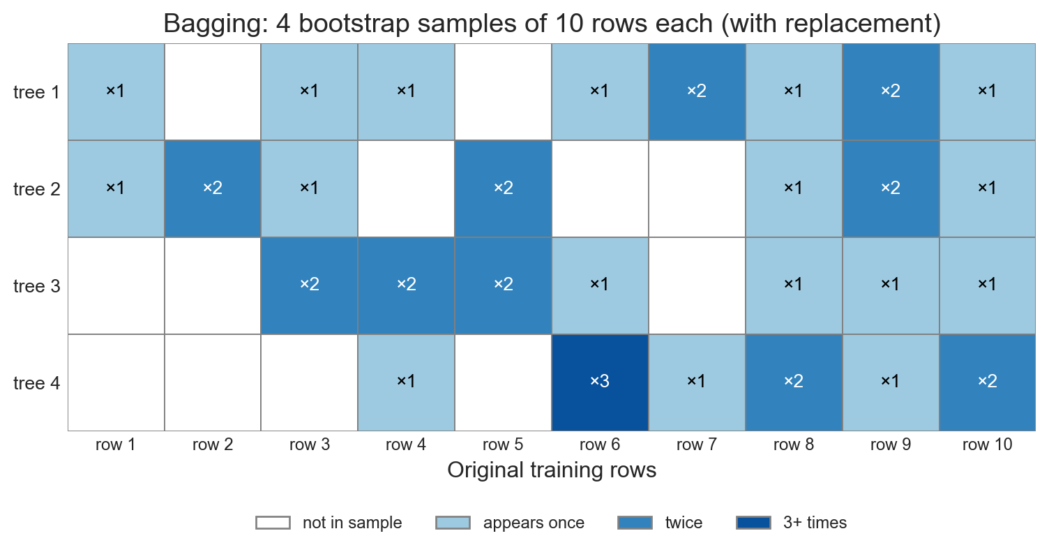
• each tree sees a different subset of rows
• some rows appear multiple times, some not at all
• skipped rows (\approx 37%) → out-of-bag (OOB) free validation

4 bootstrap samples of 10 rows each. White cells: row not in this tree’s sample. Light blue: appears once. Dark: appears 2× or 3× times.

A bootstrap of size n from n rows includes about 63% of distinct rows; the other 37% are out-of-bag (OOB) — sklearn can use them for free CV (oob_score=True).

Galton, Vox Populi (1907)

• 787 villagers at a country fair, 1906
• each guesses the weight of an ox
• guesses wildly varied — under and over by hundreds of pounds
• median guess: 1207 lb
• true weight: 1198 lb
• median within 1% of truth

“the middlemost estimate expresses the vox populi … an excellent democratic judgment.”

Galton, “Vox Populi”, Nature 75, 450–451 (1907)

can the same idea work on overfit trees? — see next slide

The Galton story. 1906 country fair, 787 entries in a guess-the-ox-weight contest. Individual guesses scatter wildly (some 100s of lb high, some 100s low) but the median sat at 1207, just 9 lb under the actual 1198 — accurate within 1%.

Galton’s 1907 Nature paper is “Vox Populi” — the wisdom of the crowd. Bagging is the algorithmic analogue: each tree memorizes different noise from its own bootstrap, and averaging shrinks the spread toward the truth.

This is the wisdom-of-the-crowd hook for the bagging argument that follows.

bootstrapped trees vs. their average

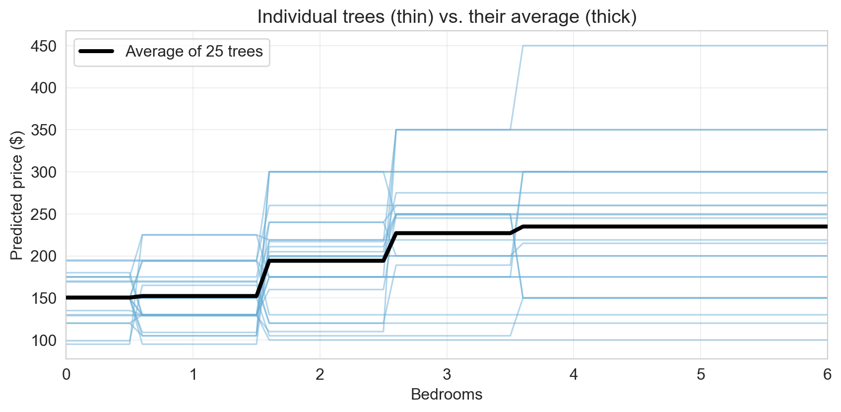
• thin blue: 25 deep trees, each fit on its own bootstrap sample
• thick black: the average prediction
• where individual trees disagree, disagreements partly cancel

25 deep trees (thin blue) — each one fit on its own bootstrap sample of rows — predicting price along the bedrooms slice (other features held at their median). They swing all over the place. The thick black line is their average: much steadier.

Visual evidence that the wisdom-of-the-crowd story from Galton works on trees: individuals are noisy, the average is calm.

Next slide quantifies “calmer.”

variance shrinks with B

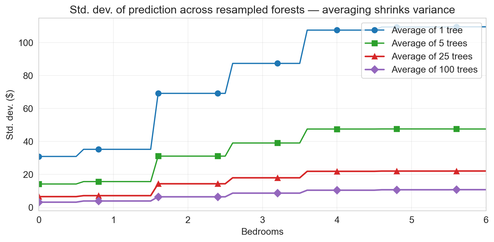
• each 4\times more trees → half the spread
• curves bend toward a floor

Same experiment, repeated for forests of different sizes B = 1, 5, 25, 100. For each B, draw a sample of B trees, average their predictions, and record the standard deviation across many such samples.

Each 4× more trees roughly halves the standard deviation — that’s the variance-of-an-average shrinking like 1/B for the noise component.

The floor that the curves bend toward is set by the average pairwise correlation between trees. Feature subsampling beats that floor down by forcing trees to consider different features at each split.

why feature subsampling matters

variance of the average of B trees, with per-tree variance \sigma^2 and pairwise correlation \rho:

\text{Var}(\bar f_B) = \rho \sigma^2 + \frac{1 - \rho}{B}\sigma^2

• the (1-\rho)\sigma^2/B term shrinks like 1/B — what averaging buys
• the \rho\sigma^2 floor doesn’t depend on B — only on how correlated the trees are
• feature subsampling lowers \rho — beats the floor down

The variance-of-an-average formula. Two terms:

1. (1 - \rho)\sigma^2 / B: shrinks like 1/B in B (so SD shrinks like 1/\sqrt{B} — what the bottom panel of the previous slide plots).
2. \rho \sigma^2: a floor that doesn’t depend on B. As long as the trees stay correlated, you can’t average your way to zero variance.

Feature subsampling pushes \rho down by forcing different splits in different trees. That’s the only lever for the floor.

Skip if running short — comes back in Ch 17 with boosting. The picture on the previous slide carries 80% of the lesson.

predict: more trees, more overfit?

we sweep the forest from B = 1 to B = 500 trees on Airbnb.

does test R^2 keep climbing forever, hit a ceiling, or U-curve?

raise hands.

INLINE PREDICT (30 sec). Quick polling/hands. Three options:

1. keeps climbing — wrong; bias is set by individual-tree depth
2. hits a ceiling — correct (slide 26 reveals the staircase)
3. U-curves — wrong; bagging has no overfitting-from-too-many-trees mechanism

The trap: students transfer the depth U-curve from Block 1 to n_estimators. The whole point of the next slide is that they’re different knobs — depth is the bias-variance lever, B is the variance-only lever.

Reveal on the next slide.

more trees rarely hurt

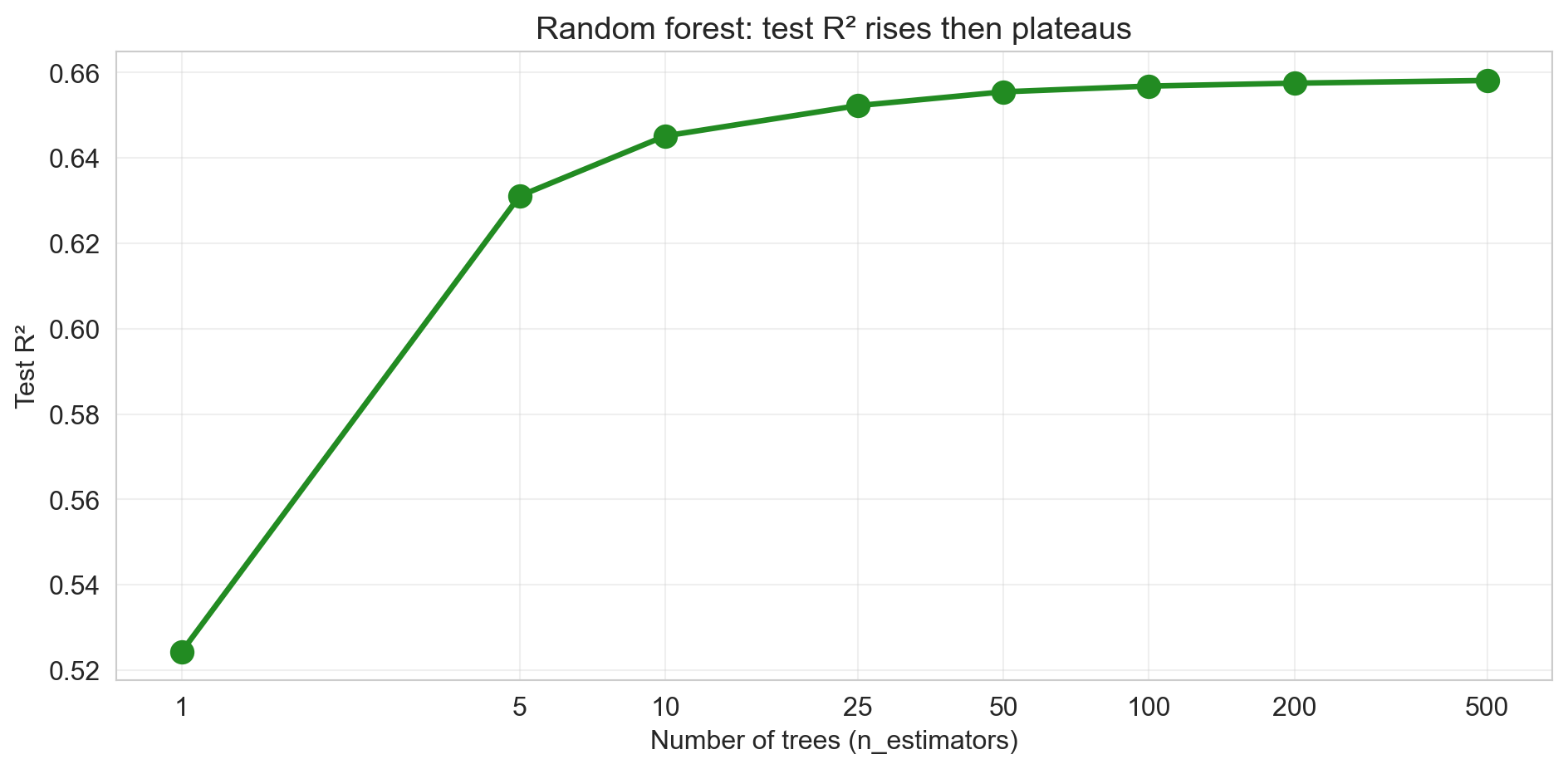
• no U-curve in n_estimators — staircase replaces the bias-variance tradeoff
• depth is the bias-variance lever, B is variance-only

Test R² as a function of n_estimators. Numbers from the chapter: 1 tree (0.524), 5 trees (0.631), 10 (0.645), 25 (0.652), 50 (0.656), 100 (0.657), 200 (0.658), 500 (0.658). Rises and plateaus. Tiny dips can happen from finite-sample noise.

This is the “one known escape” promised by Ch 6. The classical U-curve assumes you fit a single model; a forest is an average over hundreds. Adding more trees drives variance down without raising bias — a one-sided staircase replaces the U-curve.

Caveat (later slide / Ch 17): this is specific to bagging. Gradient boosting can overfit if you add too many trees because each new tree corrects errors of earlier ones — different mechanism.

About 1 min.

the surprise

test R^2 comparison

model	test R^2
linear (bedrooms + bath + room + borough)	0.571
linear + bedrooms × borough interactions	0.576
decision tree (depth 4)	0.559
random forest (100 trees)	0.657

forest improves R^2 by 0.08 over hand-engineered linear — with no manual feature engineering

The chapter’s surprise lands here. Hand-engineered linear with bedrooms × borough interactions: 0.576. Random forest, same raw feature matrix, no manual interactions: 0.657. R² improves by 0.08 (about a 14% relative improvement) on held-out data.

The forest wasn’t given the interactions — it discovered the relevant cuts on its own. That’s the answer to Friday’s brief from the opening: yes, ship the forest.

Caveat for honesty: a single deep tree at the same default depth overfits; a forest at min_samples_leaf=5 doesn’t. The bagging structure is what makes it work — not just “more trees better.”

About 90 sec — let the table sit.

the forest improves R^2 by 0.08 over the linear model.

name three reasons you might still ship the linear model.

DISCUSSION: think-pair-share (4 min). 1 min think + 2 min pair + 1 min debrief.

Tight-prompt variant of “are linear models useless?” — forces students to commit to a number (three) and defend a counterintuitive call (ship the worse-on-R² model).

Target answers — collect from class:

1. interpretable coefficients. “$1 extra bathroom is worth +$62/night, controlling for everything else.” A regulator or a host can read it.
2. odds ratios for logistic. Log-odds per feature change → multiplicative odds — the host knows what to push.
3. small datasets. Forests need lots of rows; LR works at n = 100.
4. stable extrapolation. Linear models extrapolate (cleanly or otherwise); a forest’s prediction is bounded by the training y range, so for inputs outside the training distribution it returns whichever leaf the splits route them to — often a poor proxy.
5. sparsity / lasso. Linear models can produce a small, selectable set of features; forests use everything.
6. causal-flavored interpretation under strong assumptions. Coefficient = marginal effect holding other things fixed (Ch 18).

Push for at least three. Wrap with: forests dominate prediction on tabular benchmarks; linear models dominate when you also need interpretability, small data, or extrapolation.

geometry of the data picks the model

trees vs. linear, two synthetic problems

The 4-panel: rows are problems (linear boundary on top, axis-aligned rectangle on bottom); columns are models (logistic on left, depth-4 tree on right).

Top-left: logistic on the linear problem — clean diagonal. Top-right: tree on the linear problem — staircase approximation. Bottom-left: logistic on the rectangle — fails (one hyperplane can’t enclose a box). Bottom-right: tree on the rectangle — perfect.

Each model loses on the other model’s natural geometry. The next slide closes with the pedagogical reading.

what wins where

linear models

good at smooth, monotone effects

bad at corners and thresholds

a single slope, not a staircase

trees / forests

good at corners, thresholds, interactions

bad at smooth diagonals

a slope becomes a staircase

fit both. compare held-out scores. don’t guess the geometry.

The two-card framing. Same act-card pattern as Ch 11’s “study A vs study B” slide.

Pedagogical takeaway: the right model is a property of the data, not the model family. On real data you don’t know which geometry the truth has — fit both and compare on the test set.

trees handle missing data

missing values in trees

modern tree libraries (sklearn ≥1.3, XGBoost, LightGBM) learn at each split which child to send missing-valued rows to — picking the direction that reduces the loss more. no imputation needed.

	linear regression	decision tree
missing values	break the model — must impute first	handled natively

real tabular data is mostly missing somewhere. trees skip the imputation question entirely.

Tree-based models handle missing values without analyst-supplied imputation. The split learns which direction missing rows go — pick the direction that reduces the loss more.

Why this matters: in real tabular data, missingness is the norm. Linear regression needs every row to have every feature; the analyst must decide how to impute (median, mean, model-based, …). Each imputation choice can bias the answer. Trees skip the question entirely.

Loops back to the model-selection discussion on the next slide — particularly the clinic-charts scenario, where most patients are missing 5–10 of 40 fields.

About 60 sec.

which model would you reach for first, and why?

insurance underwriter

needs one-line explanation for each premium decision

music app

wants the model to discover which combinations of behavior predict upgrades — no hand-coded rules

clinic chart coding

flag billing errors

40 fields, most patients missing 5–10

DISCUSSION: think-pair-share (5 min). 1 min think + 2 min pair + 2 min debrief.

Target answers:

1. Insurance underwriter → logistic regression. Coefficients give the per-feature explanation a regulator wants. Trees can be visualized but lose interpretability quickly past depth 3.

2. Music app → tree / forest. The hidden rule is a threshold-and-interaction pattern (genre count AND playlist count, only on some devices). A tree can discover that rule from raw signals; a linear model needs to be hand-fed the cross.

3. Clinic charts → tree / forest. 40 features with massive missingness — trees handle missing data natively (XGBoost, LightGBM, recent sklearn). Linear regression breaks without a number to multiply.

Key insight: the right model is a property of the data + decision. Interpretability requirements, missingness, sample size, and the geometry of the truth all matter.

If running short, cut to two scenarios.

what the forest used vs. what raises the price

feature importance: MDI

mean decrease in impurity (MDI)

impurity drop at a split = parent’s impurity − weighted average of children’s impurity (impurity = SSE for regression, Gini for classification)

MDI for feature j = sum of impurity drops across every split on j, weighted by samples, averaged across trees, normalized so features’ MDIs sum to 1

answers: how much does the forest use this feature?

The standard sklearn feature_importances_ output. Conceptually: which variables does the model rely on most for splitting?

The definition unpacks in two steps: 1. At one split, “impurity drop” is how much more homogeneous the children are than the parent. This is exactly what the tree was maximizing when it chose the split (greedy: minimize child impurity = maximize impurity drop). 2. For one feature, MDI accumulates the drops over every split that used that feature, weighted by the share of training rows flowing through the node — bigger nodes get more weight. Then average across trees, normalize.

Result: a feature with a few big-node splits can dominate; a feature only used at tiny leaves contributes little.

Doesn’t mean what students often hope it means (next slide).

what the forest uses

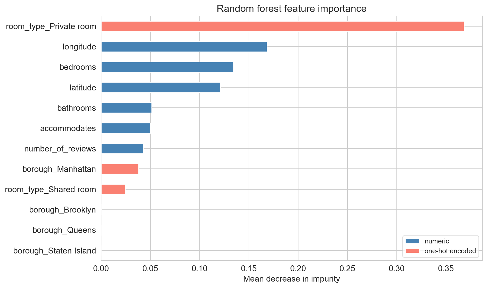
high MDI ≠ “this feature causes the outcome” — only “the forest splits on it”

The MDI bar chart on Airbnb. Top features: room_type_Private room by a wide margin, then longitude, bedrooms, latitude, bathrooms, accommodates — the room-type + geographic + size cluster.

Crucial gloss: high MDI means “the model uses this feature for splitting often”, not “this feature causes higher prices”. Location and room type are useful because they predict price, but redrawing the room_type column doesn’t make your apartment more expensive — that’s a causal claim, not a descriptive one.

Same caveat for permutation importance (next slide).

MDI vs. permutation importance

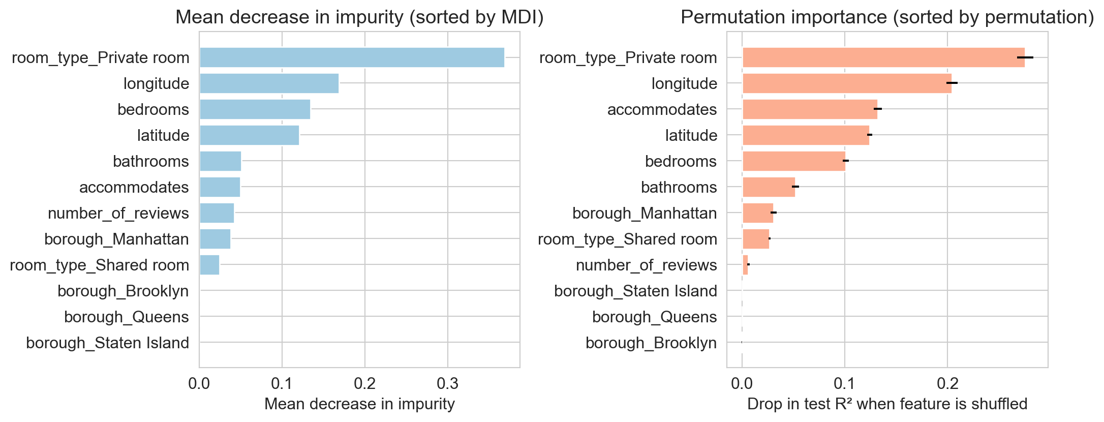
• MDI — counts split chances, biased toward continuous, high-cardinality columns
• permutation — measures held-out R^2 drop after shuffling a column, model-agnostic but slow

Two panels — same forest, two metrics, each panel sorted by its own metric. Features re-rank between the panels.

MDI bias: a continuous column has hundreds of possible split points; a binary column has one. Two equally predictive features can rank very differently just from cardinality.

Permutation importance: shuffle the column on held-out data, watch how much test R² drops. Model-agnostic, less biased by cardinality, but slow.

Two practical rules: 1. Compute permutation importance on held-out data, not training. 2. Watch correlated features. If two columns share signal, shuffling either alone can look unimportant because the model leans on the other. Drop correlated groups together.

when to doubt the forest

three failure modes

• distribution shift — predictions are bounded by the training y range; new inputs route into some leaf whose mean may be irrelevant
• importance is descriptive, not causal — high MDI on accommodates doesn’t mean adding capacity raises price
• correlated features share importance — bedrooms and accommodates: interpret as a group

Three limitations that a strong test-set R² does not address:

1. Distribution shift. Each prediction is the mean outcome in a training leaf, so the forest cannot extrapolate beyond its training data. For inputs unlike anything seen at training — new neighborhood, post-pandemic price regime — there is no nearby leaf to draw from. Same lesson as Ch 6.

2. Importance ≠ causal. Both MDI and permutation answer “what does the model use?” — not “what makes the price go up?”. Do not act on importance as a causal claim.

3. Correlated features. When two features carry overlapping signal, the per-feature importance understates each one’s real importance — the forest leans on the other when one is shuffled.

Next two slides drill into (1) and (3) with concrete demonstrations.

About 1 min for the overview; drill-ins are short.

distribution shift: linear vs. forest extrapolation

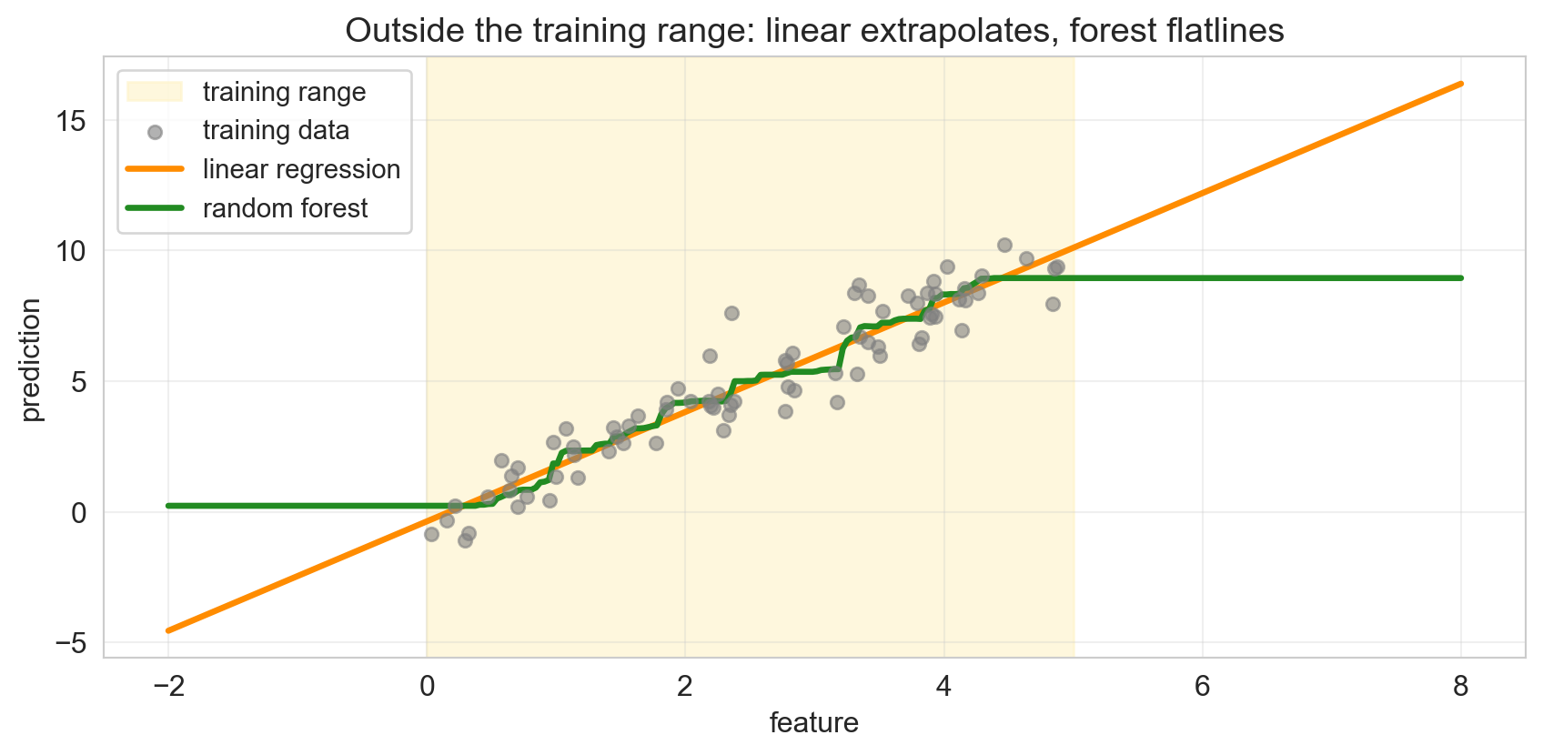
• linear extends its slope past the training range
• forest flatlines — predicts the nearest leaf’s mean

Synthetic 1D demo: training data in [0, 5] with a near-linear trend. The linear model extends the slope into [-2, 0] and [5, 8] — fine if the truth really is linear there, wrong otherwise. The forest predicts a constant outside the training range: it has no leaf for those inputs, so it returns whichever leaf the splits route them to (the boundary leaf’s mean).

Takeaway: linear extrapolation might be right or wrong; the forest’s flat extrapolation is wrong by construction — it has no information out there. Drift monitoring matters more for trees than for linear models.

About 60 sec.

correlated features hide importance

permutation drop in test R²

shuffle a feature’s column; measure how much R² drops

bedrooms and accommodates: correlation 0.64

shuffle	R^2 drop
bedrooms alone	0.10
accommodates alone	0.13
both together	0.29

with near-duplicates, each alone \approx 0; the group \gg the sum

Concrete demo. With moderate correlation (0.64), shuffling each feature individually still shows non-trivial drops — but the group drop (0.29) exceeds the sum of individual drops (0.23). Each feature’s individual permutation understates its real importance because the forest can lean on the correlated partner.

The dramatic version, mentioned on the slide: imagine an accidental duplicate column. Each individual permutation would barely move R² (the forest just uses the other copy), but shuffling both would be ruinous. Same effect, exaggerated.

Practical takeaway: interpret importance for correlated groups, not single columns. Don’t drop a feature on the basis of low individual importance if a correlated cousin is doing its work.

About 75 sec.

back to the host

Tip

Friday’s brief.

• ship the forest — improves R^2 by 0.08 over hand-engineered linear, no hand-picked interactions
• monitor distribution shift — drift on inputs; e.g., new neighborhoods, new price regimes
• don’t present importance as causal — what the model used, not what raises a price

The chapter’s closing answer to the brief. Forest goes into production. Drift monitoring on the inputs (new neighborhoods show up as feature distributions outside the training range). Don’t present the importance chart as causal to the host.

summary

• trees split automatically — find structure, no encoding, no imputation needed
• a single deep tree memorizes — train R^2 \to 1, test R^2 collapses, CV picks the depth
• random forests average overfit trees — bagging + feature subsampling, more trees rarely hurt
• trees vs. linear is a geometry choice — corners + thresholds vs. smooth slopes
• importance is descriptive — what the forest used, not what causes the outcome

Five takeaways. The first three are the technical spine; the fourth is the comparison frame; the fifth is the critical-thinking caveat that closes the chapter.

demo: trees in the notebook

colab.research.google.com/…/lec13-trees.ipynb

what to watch:

• max_depth sweep — see the U-curve happen
• n_estimators sweep — see the staircase
• swap regression for classification — same recipe, AUC (area under ROC curve, Ch 9) instead of R^2

Demo slide. The notebook has the full pipeline: load data → fit tree → tune depth via CV → fit forest → compare on test → look at feature importance. Students should run cells, change hyperparameters, watch the curves.

If running short on lecture time, point at the notebook for the bagging-variance-reduction figure (one of the most important plots; can verbally walk through if not landed on slides).

next: dimensionality reduction (Ch 14)

what if your features are already redundant?

• PCA — find directions of maximum variance
• scree plot picks the number of components
• standardization is essential — otherwise the largest-magnitude column dominates

Forward pointer. Lec 14 (Wednesday): PCA. The setup question: what if your features are correlated to start with — can you compress them to a smaller set without losing signal? PCA finds the directions of maximum variance; SVD computes them; loadings tell you which features drive each component.

Then Ch 15 takes another step into unsupervised territory with k-means clustering.

feedback

forms.gle/feedback

what worked? what didn’t? what’s still confusing?

Standard feedback slide. Same form as previous lectures.