Lecture 12: Regression Inference + Diagnostics

MSE 125 — Applied Statistics

Madeleine Udell

Wednesday, May 6, 2026

logistics

• HW 3 due Fri May 8
• project proposal feedback returned end of this week
• project midterm report due Friday May 15

START RECORDING.

HW 3 due Friday. Quiz 5 was earlier this week. Project proposals were submitted last week; feedback returned next week.

the brief

Airbnb host, NYC

$50,000 renovation for a second bathroom?

listings with more bathrooms charge more — is the premium real, large enough to recoup, stable enough to bet on?

NBA front office

analytics team’s claim: rest boosts performance — restructure the schedule around it?

before they act, let’s check: does the data support that claim?

same toolkit. very different answers.

Two parallel decision problems frame the lecture:

1. Airbnb host: clean regression, decision-grade answer (yes, do the renovation).
2. NBA front office: same machinery, finds “significance” without practical importance — and probably confounding on top.

Don’t tease the punchlines. Just frame both decisions, signal that the chapter pulls them apart, and move on. The arc lands when block 2 plays out the NBA result against the Airbnb baseline.

today

• Airbnb regression: read a regression table; t-test, CI, prediction interval
• NBA cautionary tale: significance vs practical importance, Simpson’s paradox
• diagnostics: do the assumptions hold?
• logistic regression: same template, z instead of t, odds ratios

Three blocks plus a logistic coda. The next slide gives students the three diagnostic questions that organize all of it.

three questions for every coefficient

	question	tool	doesn’t answer
Q1	nonzero?	t-test, p-value, CI excludes 0	how big
Q2	big enough?	coefficient, CI width, Cohen’s d	are assumptions met
Q3	trustworthy?	residual plot, Q-Q, LINE	confounding

we’ll walk through these questions twice:

• Airbnb answers yes to all → act on it.
• NBA shows equivocal answers → don’t act.

This is the chapter’s pedagogical scaffold. Read it slowly. Q1 is the t-test; Q2 is effect size (Cohen’s d); Q3 is diagnostics (LINE). The pivot from Q1 to Q2 is the chapter’s central pedagogy (“statistical significance is no substitute for practical importance”). The boundary at Q3 is the chapter’s second pedagogy (“diagnostics catch statistical, not systematic, problems”).

When students get lost later, this slide is the home base. The three dark transitions later in the deck are tagged to which question they’re answering.

regression for decisions

Airbnb listings, NYC

airbnb = pd.read_csv('data/airbnb/listings.csv')
airbnb_clean = airbnb[
    (airbnb['price'] > 0) &
    (airbnb['price'] <= 500) &       # filter outliers
    (airbnb['bathrooms'].notna()) &
    (airbnb['bedrooms'].notna()) &
    (airbnb['room_type'] == 'Entire home/apt')
]

n = 14,689 listings (after filtering)

Filter to entire-apartment listings under $500/night to keep the model in the regime that covers most hosts. The next slide shows the obvious bivariate patterns. Both are real but tangled — bigger places have more bathrooms AND more bedrooms, so the marginal effect of one bathroom holding bedrooms constant is what we want.

price by bathrooms and borough

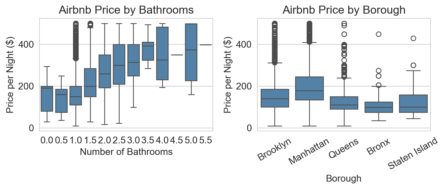
obvious patterns: more bathrooms → higher price; Manhattan > Brooklyn > rest.

but bathrooms and bedrooms are correlated.

Bivariate pictures. Both bathrooms and borough show clear patterns, but the bathrooms picture is confounded by bedrooms (more rooms → more of both). Multivariate regression is what isolates the bathroom premium holding bedrooms and borough constant.

predict before you fit

sketch your guess for two numbers in the regression below — sign and rough magnitude.

1. bathrooms coefficient ($/night per extra bathroom)
2. Manhattan vs Bronx gap ($/night)

airbnb_model = smf.ols(
    'price ~ bathrooms + bedrooms + C(borough)',
    data=airbnb_clean
).fit()

INLINE PREDICT (45 sec). Write down your guesses for the two numbers. Don’t worry about being precise — get the sign and rough scale right.

Most students will guess: bathrooms coefficient $50–$100, Manhattan-Bronx gap $50–$100. The actual answers ($62 and ~$80 respectively) are in the right neighborhood for confident guessers and a useful surprise for ones who guessed too low.

This is the first activity. Keep it brief — students need to commit to a guess before seeing the table, so the surprise of the rest-effect punchline lands when we re-run the same predict-then-reveal in block 2.

the regression table

                              coef    std err     t     P>|t|    [0.025   0.975]
Intercept                   89.0594    3.487    25.541  0.000   82.225   95.894
C(borough)[T.Brooklyn]      26.4317    3.347     7.898  0.000   19.871   32.992
C(borough)[T.Manhattan]     78.9870    3.354    23.546  0.000   72.412   85.562
C(borough)[T.Queens]        -3.6129    3.563    -1.014  0.310  -10.597    3.371
C(borough)[T.Staten Island] -8.6260    7.063    -1.221  0.222  -22.471    5.219
bathrooms                   62.4408    1.860    33.566  0.000   58.795   66.087
bedrooms                    34.0263    0.961    35.394  0.000   32.142   35.911

every regression output you’ll see has these columns. we’ll walk through bathrooms end to end, then have a template for the rest of the course.

Display the actual model.summary() output. Five columns per coefficient row, plus header (R², F) and footer (Cond. No.). Don’t try to teach all eight elements at once — the next slide takes the bathrooms row and walks through the five columns; the rest of the table fills itself in.

The intercept is “predicted price for a Bronx 0-bath 0-bed listing” — $89, which is a bit low for a 0-bath listing (the row is sparse, intercept’s there for the formula). Borough coefficients are gaps relative to Bronx (the alphabetically-first level dropped as reference).

reading the table: 5 columns per row

column	what it answers	bathrooms
coef	\hat\beta_j	$62.44 / bath
std err	how precise?	$1.86
t	\hat\beta / \widehat{\text{SE}}	33.6
P>|t|	reject H_0: \beta=0?	< 0.001
[0.025, 0.975]	95% CI	[$58.80, $66.09]

plus header: R^2 = 0.40, footer: Cond. No. = 35

Five columns walked through with the bathrooms numbers in the right column. The $62.44 / bath coefficient is the headline. SE $1.86 means we know that number to within a few dollars. t = 33.6 is enormous (far above the |t| > 2 threshold). p < 0.001. The CI [$58.80, $66.09] excludes zero by a country mile and is narrow enough to drive a renovation decision.

Header: R² = 0.40 means the three predictors explain 40% of price variance. Cond. No. = 35 is just over the multicollinearity threshold (30) — bathrooms and bedrooms ARE correlated, expected. Not a problem.

Footnote: the F-statistic is also in the header. We don’t lean on it in this course — when each individual coefficient already has its own t-test, the omnibus version rarely changes a decision. Just know it exists.

About 90 sec on this slide.

interpreting the coefficients

• bathrooms ($62): each extra bathroom → ~$62 more per night, controlling for bedrooms and borough
• bedrooms ($34): similar story; smaller premium
• Manhattan vs Bronx (+$79): the borough premium
• Brooklyn vs Bronx (+$26): closer to Manhattan than to outer boroughs
• Queens, Staten Island: not distinguishable from Bronx at \alpha=0.05

“holding everything else constant, a one-unit increase in x_j is associated with a \hat\beta_j change in y”

Walk through the signs. Most are unsurprising; the Brooklyn premium being smaller than Manhattan is the obvious geographic story. Queens and Staten Island not significantly different from Bronx is a function of (a) sample size in those boroughs and (b) actual similarity in the cheap end of the price range.

The “holding everything else constant” gloss matters: this is what students should understand by “controlling for.” The next slide makes the warning explicit.

Note: the intercept ($89) is the “Bronx 0-bath 0-bed listing” prediction — useful for the formula, not for interpretation.

would adding a bedroom raise YOUR listing price by $34?

think about what changes when you add a bedroom to your apartment.

DISCUSSION: think-pair-share (4 min). 1 min think; 2 min pair; 1 min debrief.

Goal: get students to see that the regression coefficient is an across-listings association, not a personal intervention prediction. Adding a bedroom usually means the apartment is bigger (more sq ft) which means many things change at once: layout, comp set, possibly higher cleaning fees, etc. The coefficient picks up the entire correlation — it’s not isolating “bedroom” as a treatment.

If stuck: “what does adding a bedroom usually require?” — bigger apartment, different building stock, etc.

Key insight: an across-listings association is not a counterfactual claim about your unit. The coefficient says “listings with more bedrooms charge more”; it does not say “adding a bedroom would lift this listing’s price.” We’ll come back to this distinction in Ch 18 with DAGs.

This is the central “association vs causation” beat for the chapter. Make sure it lands before moving on.

the conditional null

coefficient null hypothesis

H_0: \beta_j = 0 \quad \text{vs} \quad H_a: \beta_j \neq 0

predictor j contributes nothing given the other predictors in this model

• conditional, not unconditional
• same predictor: significant in one model, not in another
• saw it in Ch 5: bathrooms coef shrank once bedrooms entered

Read the null carefully: it’s a conditional statement. The same variable can fail in one model and pass in another. Students saw exactly this in Ch 5 — the bathrooms coefficient was larger before bedrooms entered the model, because some “bathroom” signal was actually apartment size leaking through.

Critical for the NBA section coming up: REST_DAYS is “significant” given player quality, opponent strength, home/away. The null we’re testing is NOT “rest days are unrelated to game score” but “rest days add nothing beyond what player quality and the other controls already explain.”

the t-statistic — Gosset, again

coefficient t-test

t = \frac{\hat\beta_j}{\widehat{\text{SE}}(\hat\beta_j)}

ratio of an estimate to its estimated SE

• exactly Gosset’s situation from Ch 10
• estimating the SE → fatter tails → Student’s t
• n large here (\approx 15{,}000) → t^* \approx 1.96
• read p-values off a normal in practice

Gosset (Ch 10) faced the same problem: when you estimate the SE from data instead of knowing it, the test statistic has heavier tails than a standard normal. Same correction here — under the LINE conditions the ratio is exactly t_{n-p-1} — but with sample sizes in the tens of thousands, the correction is invisible.

If asked about df: it’s n − p − 1 (one per estimated parameter, including the intercept). This goes in the Going-deeper box of the book.

Multiple-testing aside: a regression with p predictors runs p tests at once, so Bonferroni/BH applies in principle. Here all our p-values are < 0.001 so the correction doesn’t change conclusions, but for marginal p-values (~0.01–0.05) it would.

CI for the bathrooms coefficient

formula: \hat\beta_j \pm t^* \cdot \widehat{\text{SE}}(\hat\beta_j)

plug in: 62.44 \pm 1.96 \cdot 1.86 = [\$58.80,\ \$66.09]

bootstrap (Ch 8) on 1,000 resamples agrees:

formula CI:    [$58.80, $66.09]
bootstrap CI:  [$58.78, $66.04]

$59–$66 per bathroom is the range we’re betting on.

The CI is the decision-grade output. Width ~$7 is tight enough to use; the lower bound $59 is large enough to clear a renovation hurdle.

Bootstrap agreement is the sanity check: if the formula and the bootstrap disagree, the LINE conditions are likely violated (we’ll check in block 3).

Note the t* ≈ 1.96 plug-in: at n = 15,000 the t critical value matches the normal to four decimal places, so we use the familiar 1.96.

decision: invest $50K?

• bathroom premium: $59–$66 / night (95% CI)
• typical occupancy: ~70% × 365 = 256 nights/year
• incremental revenue: ~$15,000–$17,000 / year
• payback: ~3 years

yes, the data support the renovation. but two caveats —

• association ≠ intervention: across-listings coefficient may overstate what adding a bathroom does
• diagnostics: does the regression’s promise of \pm 1.96 \cdot \text{SE} actually hold? (block 3)

The point of an entire block on Airbnb: a regression with a tight CI and a meaningful magnitude IS decision-grade in many real settings. The point of a stats course: don’t sell the decision without the caveats. Block 3 will check whether the CI is honest, and Ch 18 will sharpen the across-listings-vs-counterfactual point.

About 75 min into block 1. Move to block 2.

prediction interval vs CI for the mean

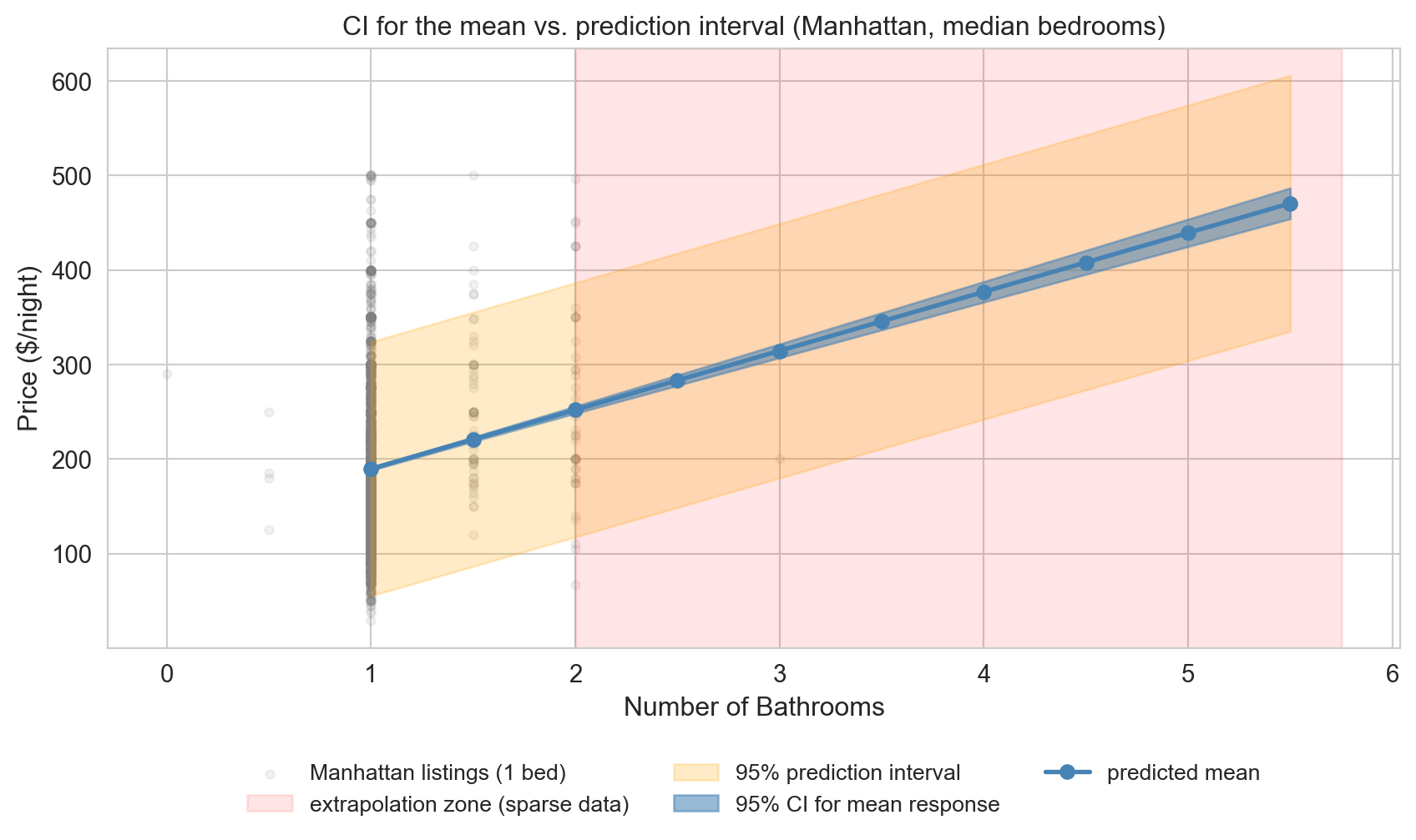
• blue band: 95% CI for the mean price at this x
• orange band: 95% prediction interval for a single new listing

PI tracks the gray scatter where data is dense; extrapolated (red shading) at high bathroom counts.

Two intervals, two questions. CI for the mean: how uncertain are we about the average price at this x? PI: where might a single new listing fall? PI is wider because it adds individual variability (\sigma^2) on top of estimation uncertainty.

The gray scatter is real Manhattan-1-bedroom listings. Where they’re dense (near 1 bathroom), the orange PI brackets most of them — exactly the job of a 95% PI. The red shading marks where Manhattan-1-bed listings barely exist (4-5 bathrooms) — the band there is extrapolated and not visually verifiable.

Forward connection: building this kind of band correctly requires the residuals to be roughly normal-shaped. The right-skew we saw two slides ago means the upper end of the orange band is too low — actual high-end listings reach the $500 cap more often than the model predicts.

NBA rest: significant, but not important

the NBA question

does extra rest help an NBA player’s game score?

what tangles a raw comparison?

• bench players get more rest (DNPs are “rest” by another name)
• stars get rested before tough opponents
• injured players return after long absences

so we control for player quality, opponent strength, home/away.

The NBA front office wants to act on a claim that rest boosts performance. Before fitting anything, we already know who is in the data is correlated with how much rest they got — the very confounders that the regression has to handle.

Set up the four-predictor model: REST_DAYS + PLAYER_SEASON_AVG + HOME + OPP_GS_ALLOWED. PLAYER_SEASON_AVG is the player’s season-long average game score (a measure of overall quality). OPP_GS_ALLOWED is the opponent’s average game score allowed (HIGH = porous defense — name flagged on a later slide).

fit, then read

model_full = smf.ols(
    'GAME_SCORE ~ REST_DAYS + PLAYER_SEASON_AVG '
    '+ HOME + OPP_GS_ALLOWED',
    data=nba_games
).fit()

                       coef     std err      t       P>|t|     [0.025  0.975]
Intercept              -0.0072  0.071    -0.101    0.919     -0.146   0.131
REST_DAYS              -0.1531  0.022    -7.020    0.000     -0.196  -0.110
PLAYER_SEASON_AVG       1.0163  0.005   192.471    0.000      1.006   1.027
HOME                    0.5022  0.057     8.764    0.000      0.390   0.614
OPP_GS_ALLOWED          1.0049  0.011    87.953    0.000      0.982   1.027

REST_DAYS: \hat\beta = -0.15, p < 0.001. statistically significant. done?

n = 72,156 player-game observations. The REST_DAYS row clears every threshold the t-test cares about: |t| = 7, p < 0.001, CI [−0.20, −0.11] excludes zero comfortably. By the criteria of block 1, we should report this as a real finding.

Don’t reveal the punchline yet — let students sit with “the data say rest hurts performance, p < 0.001” for a moment. Block 1 said a tight CI excluding zero meant decision-grade. Here, taking that seriously would say “rest hurts; cut rest days.” That conclusion is wrong, and the next slide tells you why.

but check the size

rest_coef = -0.153          # game score points / extra rest day
game_score_std = 7.85       # SD of game score across player-games
cohens_d = rest_coef / game_score_std

Cohen's d = -0.0195 SD

Cohen’s d

coefficient divided by response SD — how many SDs of the outcome does a one-unit predictor change move the prediction

Cohen’s d puts the coefficient on a unitless scale. Here -0.02 — a fiftieth of a standard deviation. The Cohen convention (small = 0.2, medium = 0.5, large = 0.8) treats this as essentially zero on any benchmark.

The slide is the formal definition. The next slide reveals the crucial pedagogical point: with n in the tens of thousands, the t-test sees this 50× more precisely than the magnitude warrants. Significance is not importance.

Cohen’s benchmarks are conventions, not laws — context matters. A tiny effect on something high-stakes (mortality) can matter; a “large” effect on something low-stakes can fail to. Here our effect is small AND on something low-stakes; both ways out fail.

significance ≠ importance

	NBA REST_DAYS	Airbnb bathrooms
coefficient	-0.15	$62.44
p-value	< 0.001	< 0.001
95% CI excludes 0	yes	yes
Cohen’s d	-0.02	0.30
practically meaningful?	no	yes

“statistical significance is no substitute for practical importance.”

Side-by-side comparison makes the lesson concrete. The first three rows are identical (both clear every textbook bar). The fourth row is the dividing line — Cohen’s d is 15× larger for bathrooms. The fifth row is the decision.

The aphorism caps the block. With n in the tens of thousands, the t-test is sensitive enough to flag effects too small to act on. Always report effect size alongside p-value.

a sports analytics team comes to you and says:

“we ran a regression and found a negative coefficient for rest days — extra rest hurts performance, p < 0.001”

before they act, what questions should you ask?

DISCUSSION: think-pair-share (5 min). 1 min think; 2 min pair; 2 min debrief.

Target answers (collect from class):

1. how big is the effect? Tiny — Cohen’s d ~ 0.02, effectively zero.
2. is there confounding? Yes — coaches choose when to rest based on schedule, opponent strength, fatigue, and recent game outcomes. The “treatment” assignment is not random.
3. does the model capture all relevant factors? No — schedule difficulty, travel, fatigue history, injury status are not all measured.
4. would this hold out of sample? Uncertain — across-season generalization needs separate validation.

Most students will land on #1 (size) and #2 (confounding) quickly. Push for #3 (omitted variables) and #4 (out-of-sample generalization). #2 sets up Simpson’s paradox, #3 sets up “Association ≠ Causation,” #4 sets up Ch 16 backtesting.

Key insight to debrief: a tight CI does not protect you from any of these. CIs widen with sample noise, not with confounding or model misspecification. Ch 18 formalizes confounding via DAGs.

standardized coefficients

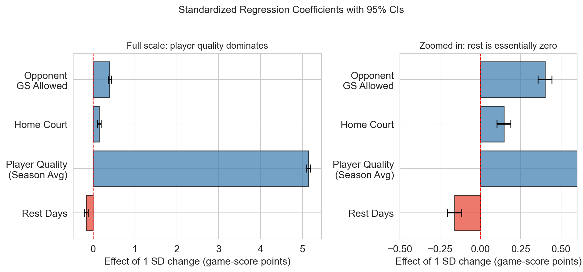
player quality dominates. REST_DAYS barely clears zero.

Standardize each coefficient by multiplying by the predictor’s SD — puts all effects on a common “per 1 SD” scale and lets you eyeball relative importance. Player season average dominates (CI bar far from zero). Home court is a small but visible bump. Opponent’s GS allowed is also large, but mechanical (next slide). REST_DAYS is the sliver at the bottom — barely clears zero, with a CI that just touches zero.

The bar that should drive a strategic decision is invisible next to the bars for variables we already understood.

variable names can deceive

we called it OPP_GS_ALLOWED = mean game score players post against this opponent

• high value = porous defense (opponents post big numbers)
• low value = stingy defense

coefficient: +1.00 — facing a porous defense → higher game score.

This is the OPP_GS_ALLOWED warning from the chapter. The variable name lied about the direction of the encoding — high “strength” actually means weak defense. The positive coefficient is mechanical, almost tautological (the regression is partly fitting “your score is your opponent’s GS allowed plus deviations”).

Real-world version: a teammate names a column ambiguously, you read the regression, the sign surprises you, you write it up — and the surprise is just a sign convention you missed. Always look at how the variable was computed before interpreting.

Also flag: same in-sample-mechanical issue affects PLAYER_SEASON_AVG (coefficient near 1 because the season average IS partly the game we’re predicting).

confounding made visible

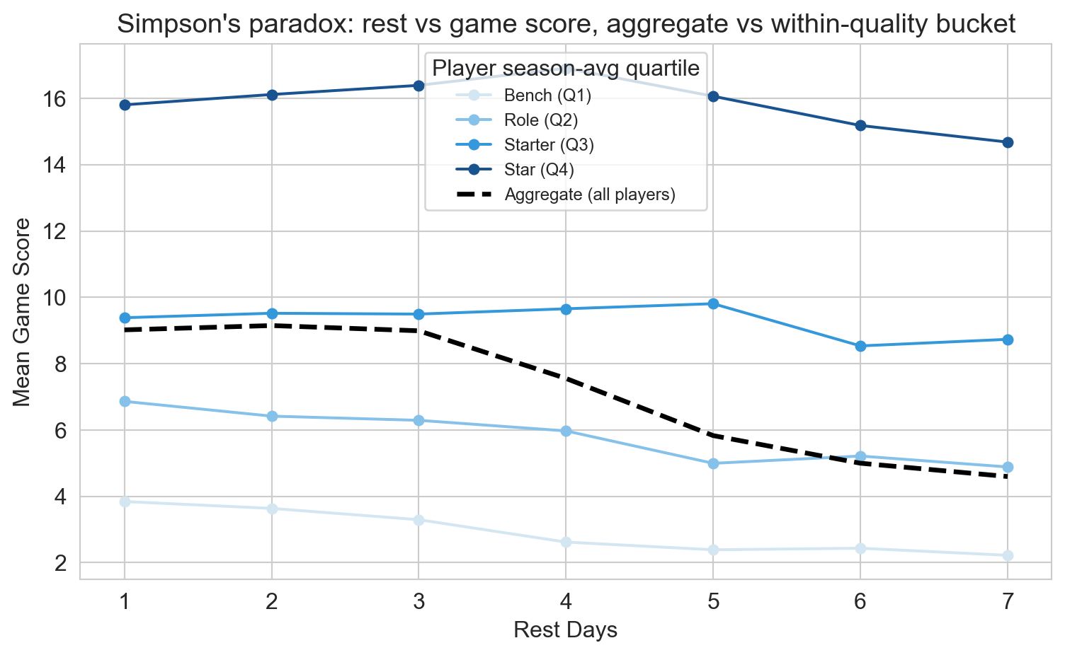
aggregate slope (dashed) steeper than within-quality slopes (colored).

adding PLAYER_SEASON_AVG is the algebraic version of switching from the dashed line to the colored ones — Simpson’s paradox in regression form.

The Simpson’s-paradox visualization. Dashed black line: aggregate trend (rest vs game score, all players). Colored lines: same trend within each player-quality quartile. The within-bucket slopes are nearly flat — once you compare like-to-like, extra rest barely moves game score. The aggregate slope is much steeper, because it picks up the compositional effect (bench players score low AND get more rest).

Strictly speaking this is the attenuation form of Simpson’s paradox: signs don’t flip, but the aggregate magnitude is much larger than any within-bucket magnitude. The lesson is the same: an unadjusted regression of game score on rest days alone would have reported a misleadingly bigger coefficient.

This visual does what the model-by-model coefficient progression in the book does — show that controlling for player quality is what isolates the rest effect.

association, not causation

regression controls for measured covariates. it does not estimate causal effects.

coaches choose when to rest:

• DNP after a soft loss ≠ DNP before a back-to-back
• rest before a tough opponent ≠ rest before a cupcake

The chapter’s “Association, not causation” warning. Coaches choose when to rest players for strategic reasons we cannot observe. Even with all the measured controls, the rest coefficient mixes the rest effect with the strategic-scheduling effect.

Forward to Ch 18: DAGs let you draw which paths a regression closes (variables you measured and controlled for) and which it leaves open (unmeasured confounders). Today’s chapter handles measured confounders well; unmeasured ones need the DAG framework.

About 75 min into block 2. Move to block 3.

Q3: is the inference trustworthy?

LINE conditions

LINE

assumptions for OLS inference:

• L linearity
• I independence
• N normal residuals
• E equal variance (no heteroscedasticity)

each letter has a diagnostic signature. residual plot covers L and E; Q-Q plot covers N; I needs you to ask whether rows are clustered.

LINE is the standard mnemonic. Pronounce it slowly the first time. The chapter introduces residual plots in Ch 5 informally; here we’re using the same plots for a sharper purpose — deciding whether the t-tests and CIs we just computed are honest.

Independence is the trickiest letter to check from residual plots alone. Both our datasets have an issue: NBA repeats players (correlated within player); Airbnb clusters by host (correlated within host). The fix is clustered standard errors. With n in the tens of thousands, clustering would widen the CIs but not flip any “significant vs not” calls — qualitative findings hold.

residual plots: do residuals have constant spread?

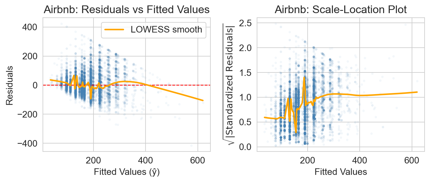
Airbnb: spread fans out as fitted price grows (“funnel”). mild heteroscedasticity.

Left panel: residuals vs fitted values. Right panel: scale-location (sqrt|standardized residual| vs fitted), which is the cleanest view of variance.

The orange LOWESS smoother on the scale-location plot trends upward — variance grows with predicted price. Expensive listings vary more in absolute dollars than cheap ones. This is a textbook E-violation, and it has a textbook fix: log-transform price.

For inference on the bathrooms coefficient, this matters less than it might seem at smaller n: with n = 15,000, the CLT still buys us approximately correct CIs on the coefficients. But a prediction interval for an individual listing’s price would be misshapen at the high end.

Q-Q plot: are residuals normal?

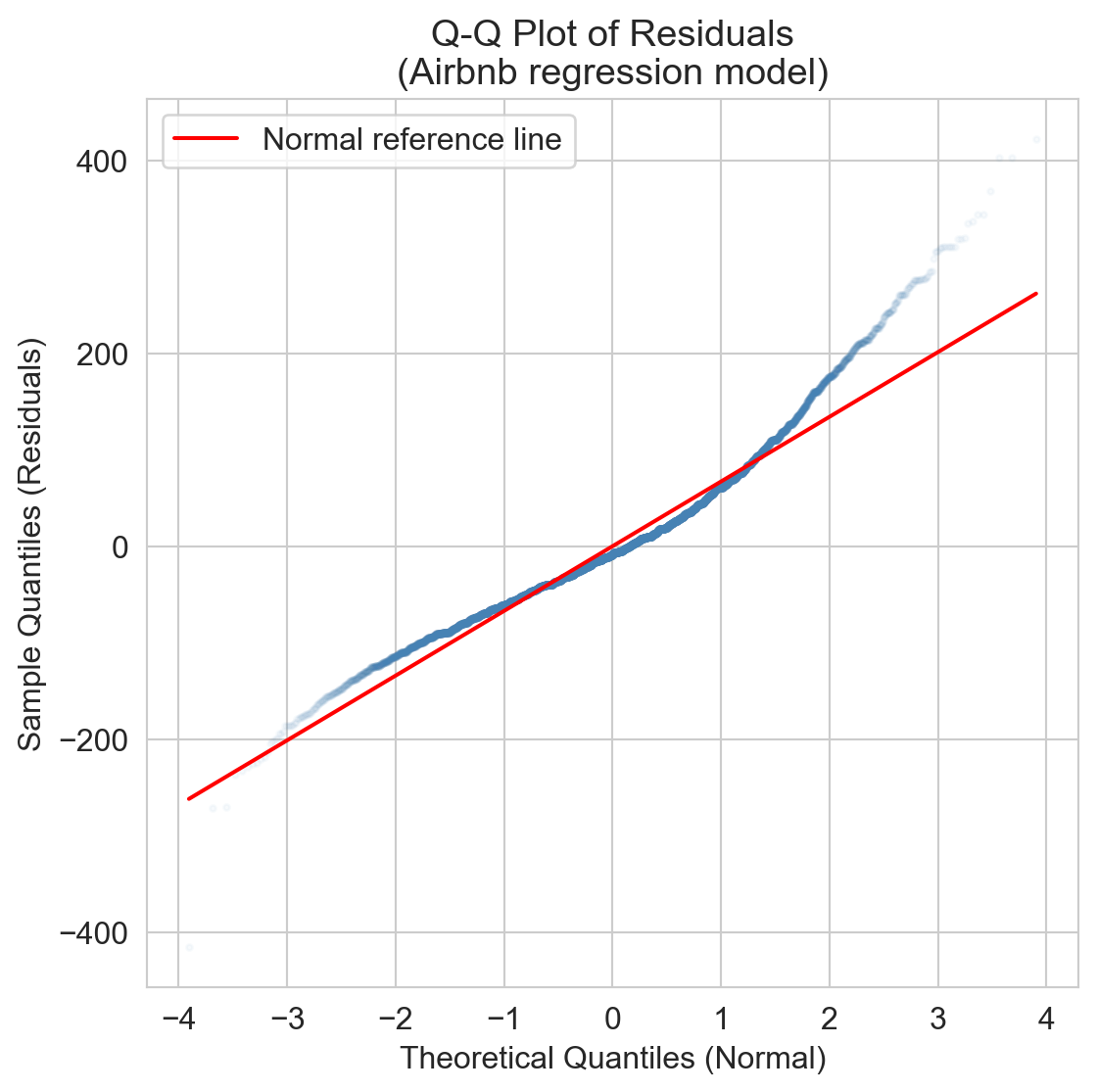
Airbnb residuals are right-skewed: prices have a hard floor at $0 but a long right tail. fix: log-transform price.

Q-Q plot compares residual quantiles to a normal. Points on the diagonal = normal residuals. Bowing up on the right = right-skew.

Airbnb: prices have a hard floor at $0 but a long right tail. Combined with the heteroscedasticity above, log price would clean both up.

NBA shows a similar but milder pattern (covered in the chapter’s Going-deeper box). The Q-Q gallery — six residual distributions matched to their Q-Q signatures — is also there for reference.

CLT covers us at n = 15,000–72,000 for coefficient CIs. Prediction intervals would underestimate the upper end.

diagnostics catch statistical problems, not systematic ones

Warning

residual plots, Q-Q plots, and the LINE conditions catch statistical problems: non-normality, heteroscedasticity, the wrong functional form

they do not catch the systematic problems that bias a coefficient as an answer to a causal question:

• selective treatment assignment
• omitted variables
• model misspecification you haven’t checked

CIs widen with sample noise or omitted variables.

they do necessarily widen with confounding.

The chapter’s strongest single sentence. The NBA REST_DAYS coefficient is the canonical case — its CI is statistically tight (n > 70{,}000), the residual plots are mostly clean — yet the coefficient would still be the wrong answer to “should we rest players more?” if rested players were also strategically scheduled against weaker opponents. Confounders bias the point estimate; they don’t show up in the SE.

This is the bridge to Ch 18. Diagnostics are necessary but not sufficient. A regression can pass every LINE check and still be answering the wrong question.

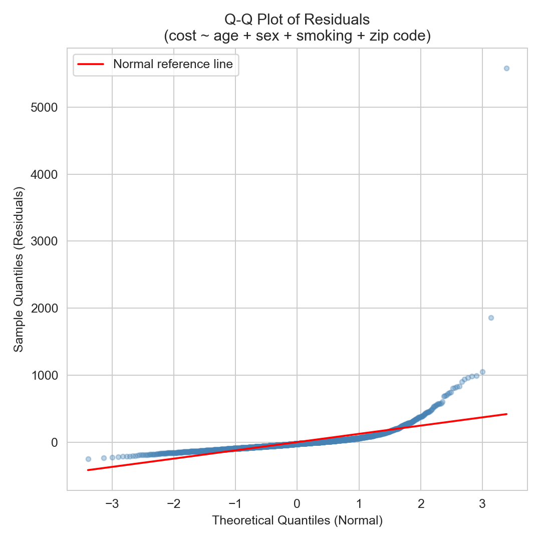
you fit a regression for monthly health-insurance claim costs:

cost ~ age + sex + smoking + zip code.

the Q-Q plot of residuals is on the right.

which LINE assumption is failing?

which fix would you try first?

DISCUSSION: analyze-this (5 min). 30 sec think; 2 min pair; 2 min debrief.

Diagnostic exercise. Right-skewed Q-Q: residuals match the normal line on the left side, then bow above it on the right — a small number of very large positive residuals. This is the N violation; common in cost data because of a small number of catastrophic claims.

Standard fix: log-transform the response (insurance cost). After log, residuals usually look more normal; coefficients become “fractional change in cost per unit predictor” rather than “dollar change.”

Probe: would clustered SEs help? Not for normality — clustering addresses I (independence). Probe: would adding more predictors help? Possibly for L, not for N directly.

If stuck: “look at the right tail — what kind of cost distribution has heavier-than-normal tails?” Insurance, asset returns, claim sizes — all right-skewed.

Key insight: each LINE letter has a characteristic Q-Q signature; matching the signature to the violation tells you what to fix. Diagnostics are a toolkit, not a binary “passed/failed” judgment.

(If the slides are running short on time, skip to the logistic coda; this discussion can be cut.)

inference for logistic regression

logistic regression: same recipe

from Ch 7: logistic models a binary outcome via the log-odds.

linear regression	logistic regression
t = \hat\beta_j / \widehat{\text{SE}}	z = \hat\beta_j / \widehat{\text{SE}}
exact t_{n-p-1} under LINE	asymptotic normal (Wald, MLE)
coef in original units	e^{\hat\beta_j} = odds ratio
[\hat\beta - 1.96 \cdot \text{SE},\ \hat\beta + 1.96 \cdot \text{SE}]	exponentiate to get OR CI

read the table the same way; just remember z instead of t, and exponentiate at the end.

The logistic-regression coda. Two changes from OLS:

1. The test statistic is z, not t. Logistic uses MLE → Wald test → asymptotic normal. There’s no exact small-sample distribution. With sample sizes in the hundreds or thousands the normal approximation is fine; with rare-event outcomes or near-perfect separation, profile-likelihood CIs are the safer fallback.

2. Coefficients are on the log-odds scale. Exponentiating gives the odds ratio (multiplicative change in odds per unit increase in x_j). CIs on \hat\beta map to CIs on the OR by exponentiating both endpoints.

The table reading template from block 1 still works — just z replaces t and exponentiate the coefficients and CIs at the end.

Framingham — odds of 10-year CHD

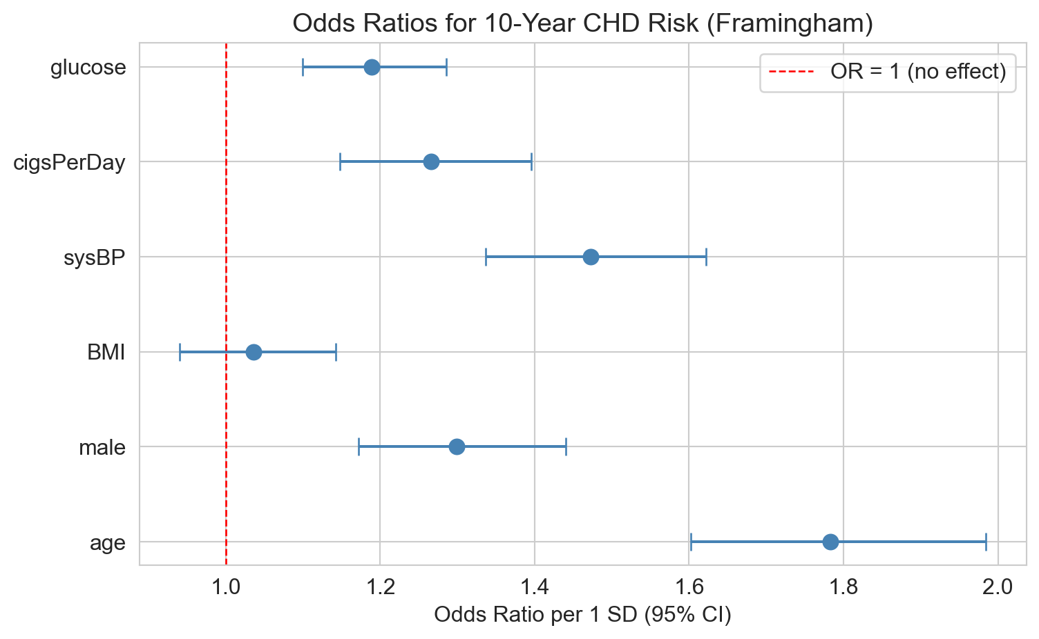
age, smoking, sysBP, glucose: OR > 1, CIs exclude 1

BMI: CI crosses 1 (not distinguishable from “no effect”)

Forest plot: each row is a predictor’s odds ratio with a 95% CI. The dashed red line at OR = 1 is “no effect.” A CI crossing 1 means the OR is not distinguishable from 1.

BMI’s CI crosses 1 — controlling for BP and glucose, BMI’s independent contribution is harder to pin down. Doesn’t mean BMI doesn’t matter; means within this model, after accounting for the other predictors, the data don’t distinguish its OR from 1.

Next slide walks through the math for interpreting the age OR.

interpreting the age OR

age \widehat{\text{OR}} \approx 1.78 per 1 SD; 1 SD of age \approx 9 years

linear in log-odds \Rightarrow multiplicative on odds

\frac{\text{odds at } x + \Delta}{\text{odds at } x} \;=\; \widehat{\text{OR}}^{\,\Delta / \sigma_x}

age 50 \to 60 is 10 years \approx \tfrac{10}{9} SD:

\frac{\text{odds}(60)}{\text{odds}(50)} \;\approx\; 1.78^{10/9} \;\approx\; 1.90

odds of CHD at 60 are about 2× the odds at 50

The pedagogy: “OR” always carries an implicit unit. The model is linear in log-odds; exponentiating gives a multiplicative effect on odds. The reported OR is per a unit change of the standardized predictor (1 SD here). To convert to a different change \Delta in the original units, raise OR to \Delta/\sigma.

Two routes to the same answer:

1. Exponentiate once: 1.78^{10/9} \approx 1.90.

2. Per-year first: \hat\beta_{\text{SD}} = \log(1.78) \approx 0.577 per SD → \hat\beta_{\text{year}} \approx 0.577/9 \approx 0.064 per year → per-year OR \approx e^{0.064} \approx 1.066 → 10-year multiplier \approx 1.066^{10} \approx 1.90.

Same answer. Route (a) is one line.

If you wanted a per-year OR directly from the fitted model, you would refit on un-standardized age — or equivalently, divide \hat\beta_{\text{age}} by \sigma_{\text{age}} before exponentiating.

summary

• Airbnb: bathrooms +$62/night, CI [$59, $66] — decision-grade. act on it.
• NBA: rest “significant” at p<0.001, but Cohen’s d \approx -0.02 — don’t act on it.
• same machinery, very different verdicts. check effect size, not just p-value
• diagnostics catch statistical problems (non-normality, heteroscedasticity), not systematic ones (confounding, omitted variables)
• logistic = same template, z for t, exponentiate the coefficients

Five takeaways. The first two are the parallel decisions. The third is the central pedagogical point. The fourth is the chapter’s strongest sentence (CIs widen with sample noise, not with confounding). The fifth is the bridge to Ch 12.5.

next: Ch 12.5 — classification meets inference

how do we ask “is this classifier real?” with the same toolkit?

• bootstrap CI for AUC — same idea as Ch 8, applied to classifier performance
• permutation test for “classifier beats random guessing”
• multiple-testing corrections over many logistic coefficients

same template throughout. only the test statistic and the response variable change.

Forward pointer to Ch 12.5. The chapter is short (15-20 min) and reuses Ch 8 (bootstrap), Ch 9 (permutation), Ch 11 (multiple testing) on classification metrics.

Then Ch 13 opens Act 3 with a completely different model family: trees and random forests.

feedback

forms.gle/feedback

what worked? what didn’t? what’s still confusing?

Standard feedback slide. The QR points to the same form as previous lectures.