Lecture 10: Hypothesis Testing

MSE 125 — Applied Statistics

Madeleine Udell

Monday, May 4, 2026

in chapter 9 we shuffled labels and got p ≈ 10⁻⁴

the drug works

but in 1991 the trial hadn’t been run yet

Open with the pivot. Last time we walked through the post-hoc analysis: data in hand, build a null distribution by shuffling, read off a tiny p-value. Easy verdict — the drug works. But that frame skips over a much harder set of questions that the people designing ACTG 175 actually faced before any patient was enrolled. Today is the prospective view: hypothesis testing as a tool for designing a study, not just summarizing one.

logistics

• project: proposal due this Friday
• quiz 5: Wed May 6 — Lec 10-11 (hypothesis testing + multiple testing)
• HW 3: due Fri May 8

START RECORDING.

Quiz Wednesday covers this lecture and next. HW 3 due Friday — uses hypothesis testing and power analysis directly. Project proposals are back — check your feedback and come to office hours if you have questions.

the design questions Ch 9 left on the table

before any data exists:

• how many patients do we enroll?
• what p-value would convince us?
• what errors are we willing to make, and at what rate?

permutation tests need data to shuffle — these questions need a formula

Three questions that all sit upstream of running the trial. None of them can be answered by shuffling, because there is no data yet to shuffle. They require a closed-form expression for the null distribution — the parametric machinery this chapter develops. Hold this transition in your head: Ch 9 was retrospective, today is prospective.

today

• the framework: \(H_0\), \(H_1\), the 4-step recipe — formalized
• two errors, not one — Type I, Type II, power
• from simulation to formula: Welch’s t-test
• power: how many patients? requires guessing the effect size
• significance ≠ importance

Five blocks. The first formalizes the vocabulary we used informally last time. Block 2 introduces the second kind of error — the one Ch 9 ignored. Block 3 makes the simulation→formula transition that lets us answer design questions. Block 4 is power analysis with a major caveat: every power calculation requires committing to an effect size. Block 5 is the failure mode that haunts every well-funded study.

the framework

the recipe

every hypothesis test, same four steps:

1. state \(H_0\) and \(H_1\)
2. choose a test statistic
3. determine the null distribution
4. compute the p-value, reject if \(p < \alpha\)

Ch 9 walked through all four with a permutation test — today we name the parts and swap step 3 for a formula

The recipe carries over from Ch 9 unchanged. What changes is row 3. Last time we built the null distribution by shuffling labels — 10,000 fake datasets each producing one fake test statistic. Today we’ll get the null distribution from a closed-form formula instead. Same recipe, different row 3.

step 1 — competing claims

for the clinical trial:

• \(H_0\): \(\mu_T - \mu_C = 0\) (no effect)
• \(H_1\): \(\mu_T - \mu_C \neq 0\) (some effect)

note: \(H_1\) is a family of effects, not a single value

a 5-cell effect, a 50-cell effect, a 500-cell effect — all live inside \(H_1\)

Two-sided alternative. Big point that we’ll keep returning to: \(H_1\) is composite. It’s the complement of \(H_0\) — every state of the world the null rules out. That includes tiny effects and huge effects and everything in between. The hypothesis test does its job without us picking any particular effect inside \(H_1\). Where it bites — as we’ll see in Block 4 — is power analysis: to compute Type II error or power, we have to pick one specific point in \(H_1\).

state \(H_0\) and \(H_1\) for each scenario

• a new website layout might increase sign-ups
• a coin might be unfair
• a pollution standard might not be met

DISCUSSION: Think-pair-share (3 min). Write \(H_0\) and \(H_1\) for all three; compare with a neighbor. Prompt: State H₀ and H₁ for each scenario. Process goal: practice translating real-world questions into formal hypotheses before we proceed. Expected answers: - Website: H₀: μ_new = μ_old (no difference in sign-up rate); H₁: μ_new ≠ μ_old - Coin: H₀: p = 0.5 (fair); H₁: p ≠ 0.5 (unfair) - Pollution: H₀: μ ≤ standard (meets the standard); H₁: μ > standard (exceeds it) If stuck: “The null is always the boring claim — nothing special is happening.” Key insight: H₀ always contains an equality. H₁ is what you need evidence to conclude. The burden of proof is on the alternative.

\(H_0\) and \(H_1\) — the formal version

null and alternative hypotheses

\(H_0\) = a single, specific claim about the world (typically “no effect”)

\(H_1\) = the complement of \(H_0\) — a family of states ruled out by the null

a hypothesis test asks whether the data are surprising enough under \(H_0\) to reject it

the test does not require us to pick a specific effect inside \(H_1\) — only to decide whether \(H_0\) is ruled out

Formalize what we did informally last time. The null is one specific value (or a single equality); the alternative is everything that null rules out — typically a whole continuum. A hypothesis test is asymmetric: we accumulate evidence against H₀, never “for” H₁ in any specific form. We reject or fail to reject — never “accept.” This asymmetry will matter in Block 2.

two errors, not one

Until now we’ve only worried about one mistake: rejecting H₀ when it’s true. There’s a symmetric mistake — failing to reject H₀ when H₁ is true — that we’ve been silent about. Both deserve names.

you’re the FDA reviewing a new drug — which mistake is worse?

• A. approve a useless drug — side effects, no benefit
• B. reject a drug that saves lives — patients die who could have been saved

DISCUSSION: Poll + debrief (3 min). Hands up for A or B (no fence-sitting); debrief by asking why students chose what they chose. Prompt: Which mistake is worse? Format: Quick hand raise (A or B), then ask 1-2 students from each side to justify. Process goal: force students to feel the asymmetry before we give it names. There’s no single right answer — depends on disease severity, the drug’s side effects, and what alternatives exist. A useless cancer drug with brutal side effects is terrible to approve; rejecting a cure for a fatal disease with no alternatives is terrible too. The point is that the two errors have different costs, and those costs should drive the choice of α. If stuck: “What if the disease is fatal and there are no other treatments? What if the drug has serious side effects?” Key insight: the two errors are not symmetric — their costs depend on context.

the courtroom analogy

think of \(H_0\) as “innocent until proven guilty”

• Type I error = convicting an innocent person
  • rejected \(H_0\) when it was actually true

• Type II error = letting a guilty person go free
  • failed to reject \(H_0\) when \(H_1\) was actually true

The single best mnemonic for the two error types. Null is innocence — the default. Evidence has to overcome it. A Type I error is a wrongful conviction: we rejected H₀ when the person was actually innocent. A Type II error is a wrongful acquittal: we let a guilty person go even though they were guilty. The justice system is deliberately asymmetric — designed to make Type I rare, even at the cost of more Type II (“better that ten guilty escape than that one innocent suffer,” Blackstone). We do the same with α.

the α-β tradeoff

\(\alpha\) = controlled directly — it’s where we draw the threshold

\(\beta\) = controlled indirectly — depends on the true effect size, which we don’t know

there is no free lunch — moving the threshold trades \(\alpha\) against \(\beta\)

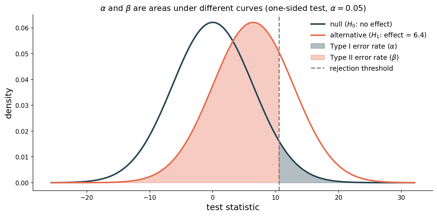
Predict-first prompt before advancing: ask students what happens to the false-positive region (under H₀) and to the false-negative region (under H₁) as the rejection threshold moves right (stricter α). Hold for 30 seconds, no hands. Then click forward — bullets reveal one at a time.

Two bell curves: null centered at zero, alternative centered at the assumed effect. Threshold is the vertical line. Blue (null past threshold) = α, the false positive rate, set directly by where we draw the threshold. Red (alternative inside the threshold) = β, the false negative rate — NOT directly controlled because it depends on how far the alternative is shifted (the true effect size, unknown). Slide the threshold right: blue shrinks, red grows. Power analysis (Block 4) computes β GIVEN an assumed effect size — that’s how we reason about β even though we can’t pin it down without knowing the truth.

the error table

	\(H_0\) true (no effect)	\(H_1\) true (real effect)
reject \(H_0\)	Type I error (\(\alpha\))	correct
fail to reject \(H_0\)	correct	Type II error (\(\beta\))

power = \(1 - \beta\) = probability of correctly detecting a real effect

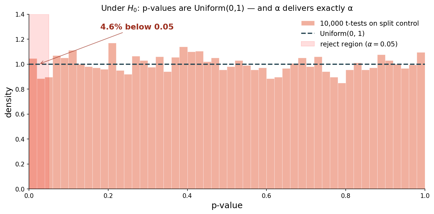
The 2×2 table. Type I rate is α — that’s by construction, since α is the threshold we set. Type II rate is β — a quantity we don’t set directly but can compute or simulate. Power is 1 − β, the probability we correctly detect a real effect. Conventional target: 0.80.

definitions — Type I, Type II, power

significance level, Type I error, Type II error, power

• significance level \(\alpha\): threshold for rejecting \(H_0\) — equals the Type I error rate
• Type II error rate \(\beta\): \(P(\text{fail to reject } H_0 \mid H_1 \text{ true})\)
• power \(= 1 - \beta\): probability of correctly detecting a real effect

Formal definitions. Notice α and β are linked: lowering α (stricter threshold) increases β (more false negatives, less power). There is no free lunch — only choices about which kind of mistake you’d rather make more often.

“fail to reject” — not “accept”

we say “fail to reject \(H_0\)” — never “accept \(H_0\)”

a non-significant result means the data are compatible with \(H_0\)

but they might also be compatible with many other hypotheses

absence of evidence is not evidence of absence

Language matters. When we fail to reject, we haven’t shown H₀ is true — we’ve only shown we don’t have enough evidence against it. Maybe the effect is real but our sample was too small. Maybe it’s real but tiny. The data are consistent with H₀ AND with a range of small effects. Einstein (reportedly): “No amount of experimentation can ever prove me right; a single experiment can prove me wrong.”

p-values are uniform under \(H_0\)

10,000 t-tests on splits of the control arm (no effect possible) → 4.6% reject at \(\alpha = 0.05\)

so \(\alpha\) does what it advertises

The empirical demonstration. Take the ACTG control group only — no treatment effect can possibly exist within it — split it randomly in half, run Welch’s t-test, repeat 10,000 times. The histogram of resulting p-values is flat: Uniform(0, 1). Any horizontal slice at α = 0.05 catches exactly 5% (here 4.6% — finite-simulation noise) of the draws below it — α delivers exactly its advertised Type I rate. Exact for exact tests (a fully enumerated permutation test); approximate for Welch’s, getting better as n grows. The flat histogram under the null is a useful sanity check when you suspect a buggy testing pipeline.

from simulation to formula

Block 3. We’ve handled the post-hoc machinery. Now: how do we get from “we have data, what’s the p-value?” to “we don’t have data yet, how do we plan the trial?” That requires a closed-form null distribution. Today’s tool: Welch’s t-test.

why a formula?

Ch 9 — null distribution by shuffling: 10,000 fake datasets, each producing one fake statistic

design question: “with 200 patients per arm and a 30-cell effect, how often will I reject?”

no data to shuffle — we need a closed-form null distribution that depends only on \(n_T\) and \(n_C\)

The transition. Permutation needs data; design questions don’t have data yet. The classical formula-based test for “do these two groups have the same mean?” is Welch’s t-test. Its null distribution depends only on sample sizes — not on actual numbers — which is exactly what design analysis requires.

the brewer who solved this in 1908

• William Sealy Gosset at the Guinness brewery, Dublin
• compared barley varieties with tiny samples (5–10 batches)
• normal approximation unreliable at small \(n\)
• couldn’t bootstrap or simulate — no computers
• so he derived the exact small-sample distribution analytically

published in 1908 as “Student” — Guinness banned real names

that’s why it’s called Student’s t-distribution

Salsburg, The Lady Tasting Tea, Ch. 2

Historical motivation, pulled before the formula. Gosset faced exactly the problem we face: small samples, normal approximation insufficient, no way to simulate. He derived the exact distribution analytically — the t-distribution. The same machinery now lets us answer design questions, where the constraint isn’t small samples but the absence of any data yet. Guinness banned real names because competitors would learn they were using statistics. The distribution has slightly fatter tails than the normal — more extreme values when you have less data — and converges to the normal as n grows.

what does t look like?

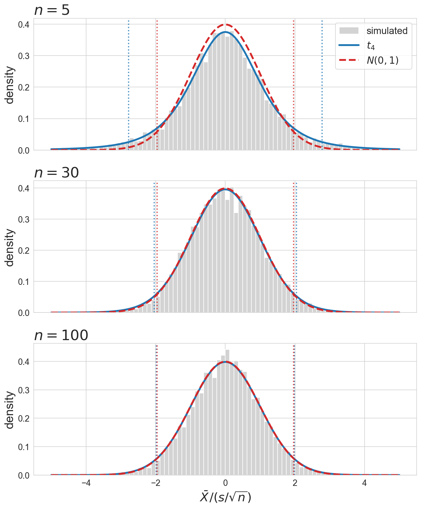
fat tails at small \(n\) — normal cutoff over-rejects under \(H_0\)

Sample \(n\) values from \(N(0,1)\), compute \(\bar X / (s/\sqrt n)\), repeat 10,000 times. At \(n = 5\) the histogram has clearly heavier tails — Gosset’s \(t_4\) tracks them exactly; the normal does not. By \(n = 30\) the two pdfs are visually indistinguishable; by \(n = 100\) everything coincides. The dotted vertical lines are the two-sided 5% cutoffs for each distribution: at \(n = 5\) the t-cutoffs sit well outside \(\pm 1.96\), so using the normal at small \(n\) over-rejects under \(H_0\). Convergence is fast: by 30 patients per arm the correction is negligible; at 5 it’s the difference between a calibrated test and a broken one.

Welch’s t-statistic

a refinement of Gosset’s that drops the equal-variance assumption — using Ch 8 notation (sample means \(\bar X_T, \bar X_C\), sample variances \(s_T^2, s_C^2\), sample sizes \(n_T, n_C\)):

\[t = \frac{\bar{X}_T - \bar{X}_C}{\left(s_T^2/n_T + s_C^2/n_C\right)^{1/2}}\]

• numerator: the observed effect (Ch 8 difference of means)
• denominator: the standard error \(\widehat{\text{SE}}\) from Ch 8

gloss: how many standard errors is the effect from zero?

Variables tied to Ch 8 notation. Numerator: difference of sample means — same statistic we bootstrapped. Denominator: the Ch 8 SE formula, plug-in estimate of the SD of the difference, with each variance divided by its own n and the two added (the groups are independent). Under H₀, this t-statistic has a known distribution — Student’s t with Welch-Satterthwaite df — that depends only on the sample sizes and variances, not on the unknown population means. That’s the engine of design analysis.

why Welch’s specifically?

two flavors of two-sample t-test:

• Student’s: assumes equal variance in both groups
• Welch’s: doesn’t

real data: variances rarely equal

equal_var=False is the safe default — use it unless you have a positive reason to assume equal variance

Pedantic but important. Both tests sit on the same t-statistic; they differ in how they compute the SE and degrees of freedom. Welch’s drops the equal-variance assumption by adjusting both. In real data, variances rarely match. Welch’s costs almost nothing when the variances are equal, and saves you from a wrong answer when they aren’t. Default to Welch’s.

Welch’s on ACTG 175

from scipy import stats
t_stat, p_value = stats.ttest_ind(
    treatment, control, equal_var=False
)
# t-statistic: 9.46
# p-value:     2.8e-19

permutation (Ch 9): \(p \approx 10^{-4}\) — limited by 10,000 shuffles

same conclusion — but the formula will also tell us what would have happened with 100 patients per arm, or 30, or 1000

Run the test. t = 9.46, p ≈ 3 × 10⁻¹⁹. The permutation p-value from Ch 9 was 10⁻⁴ — that floor is the resolution of 10,000 shuffles, not a real disagreement; both verdicts say “reject decisively.” The advantage of the formula isn’t a different answer on this data — it’s that the formula tells us what would have happened with sample sizes we didn’t run. That’s what makes power analysis possible.

A/B testing — same recipe, different stakes

a growth team tests a new homepage layout:

• variant B: 4.2% sign-ups, \(n = 12{,}400\)
• variant A: 4.0% sign-ups, \(n = 12{,}200\)

Welch’s logic, identical machinery → \(p \approx 0.04\)

Type I error: ship a feature that doesn’t help (dev cost, maintenance)

Type II error: kill a feature that would have moved the needle

most companies use a less strict \(\alpha\) than the FDA — wrong shipping decisions are reversible

The dominant industrial application of two-sample testing — and the one most MS&E students will actually run in their careers. Same machinery as ACTG: observed difference, standard error, p-value. The stakes change. Type I means shipping something useless; Type II means killing something useful. Most tech companies sit at α = 0.05 to 0.20, depending on how reversible the decision is and how much they value shipping speed. The cost ratio of the two errors should set α; the FDA and a startup land on different points of the same curve. Hold this in your head as we move to “what should α be?” next.

trial result: p = 0.04

colleague A

“just barely significant — shouldn’t be trusted”

colleague B

“p < 0.05 — we reject”

who is right? what does this reveal about the 0.05 threshold?

DISCUSSION: Think-pair-share (4 min). Think individually, then discuss with a neighbor; be ready to defend either side. Prompt: p = 0.04 — who is right? Process goal: surface the arbitrariness of α = 0.05 and the fact that p-values are continuous evidence, not binary verdicts. Both colleagues are partly right. B is correct procedurally — if you committed to α = 0.05 before seeing the data, p = 0.04 crosses the threshold. A raises the deeper point — p = 0.04 and p = 0.06 carry nearly identical evidence, yet one “rejects” and the other doesn’t. The 0.05 threshold is a convention, not a law of nature. If stuck: “Is p = 0.049 fundamentally different from p = 0.051?” Key insight: α is a decision tool, not a truth detector. Reasonable people can disagree where to set it. The right α depends on the stakes — Block 4 makes this explicit.

what should \(\alpha\) be?

field	typical \(\alpha\)	why
social science	0.05	convention (Fisher, 1925)
clinical trials	two trials, each 0.05	combined: ~0.0025
particle physics	~0.0000003	“5-sigma”

the choice depends on the cost of each error type, not on convention

The choice of α is not a statistical question — it’s a decision about how much false-positive risk you’re willing to accept given the stakes. Social science: 0.05 by convention, inherited from Fisher’s 1925 textbook. FDA: requires two independent positive trials each at 0.05, joint Type I rate roughly 0.05² = 0.0025. Particle physics: 5-sigma (~3 × 10⁻⁷) because claiming a new particle that doesn’t exist is catastrophic for the field. The two-trial FDA rule is the simplest example of a multiple-testing correction — Ch 11 generalizes.

power: how many patients?

power = the inverse question

so far: given data, what’s the p-value?

now: given a hoped-for effect, what’s the chance of a small p-value?

what study designers compute before the trial — to decide \(n\)

The pivot from post-hoc to prospective analysis. The formula we just got lets us compute, for any assumed effect size and any sample size, the probability that a t-test would reject. That probability is power = 1 − β. It tells us whether a planned study is big enough to find what we’re hoping to find.

the catch — power needs a specific \(H_1\)

remember: \(H_1\) is a family of effects

power asks: “what’s the chance we reject if the true effect is \(\Delta\)?”

different \(\Delta\) → different power

so: we have to commit to a specific effect size to compute one number

The conceptual hinge of the chapter. The hypothesis test itself runs without us picking any specific effect inside H₁ — we just check whether the data are surprising under H₀. But power and Type II error are defined relative to a specific point in H₁: we’re asking how often we’d correctly reject if the world is in that state. Different states give different powers, so we must pick one to compute one number.

what does picking \(\Delta\) mean?

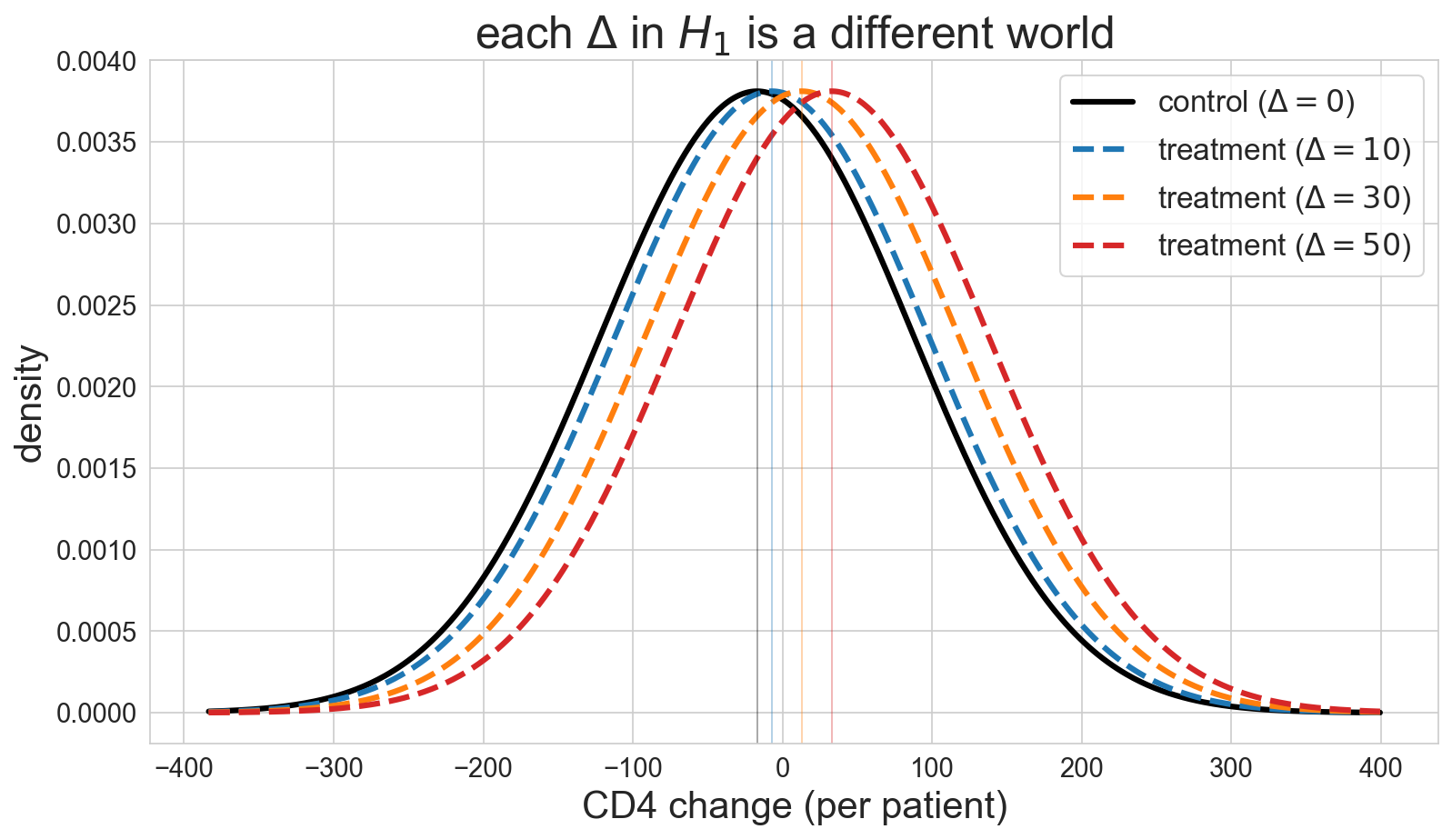
each \(\Delta\) = a different world we might be in

bigger \(\Delta\) → populations farther apart → easier to detect

The visualization that makes “effect size” concrete. Control distribution centered at the population mean. Three treatment distributions shifted by 10, 30, 50 CD4 cells. With σ ≈ 105 of patient-to-patient variation, even Δ = 50 leaves the distributions heavily overlapped — knowing one patient’s CD4 change tells you almost nothing about which arm they were in. What rescues us is sample size: the SAMPLING distribution of the DIFFERENCE OF MEANS shrinks as n grows, so even small Δ can become detectable with enough patients.

you must guess the effect size

no effect size, no power analysis

power = \(P(\text{reject} \mid \text{true effect} = \Delta)\) — needs a value of \(\Delta\)

where the guess comes from:

• prior studies of similar interventions (most defensible)
• the smallest effect that matters clinically or commercially
• a pilot study designed to estimate plausible effects

doubling the assumed effect cuts required \(n\) by roughly 4×

The guess is unavoidable, and it dominates the answer. Sample size scales like 1/Δ², so doubling the effect cuts n by 4× — and that sensitivity is exactly why reviewers always scrutinize the assumed effect in published trial protocols. If you’re an analyst doing power analysis: be explicit about where your effect-size assumption comes from. If you’re a reader of a study: that’s the first thing to interrogate.

predict — how much power?

true effect = 30 CD4 cells, 100 patients per arm

what fraction of trials correctly reject \(H_0\)?

90%? 75%? 50%? 25%?

0.5 — a coin flip

that’s an underpowered study

The surprise. Most students guess 80% or higher because 100 patients sounds like a lot. The actual answer is 0.5 — the trial is roughly as informative as flipping a coin. The reveal is the lesson: sample size requirements for plausible HIV effects are much larger than student intuition predicts. Hold this in head when the power curves arrive next — the 30-cell line crosses 0.8 only past n ≈ 200.

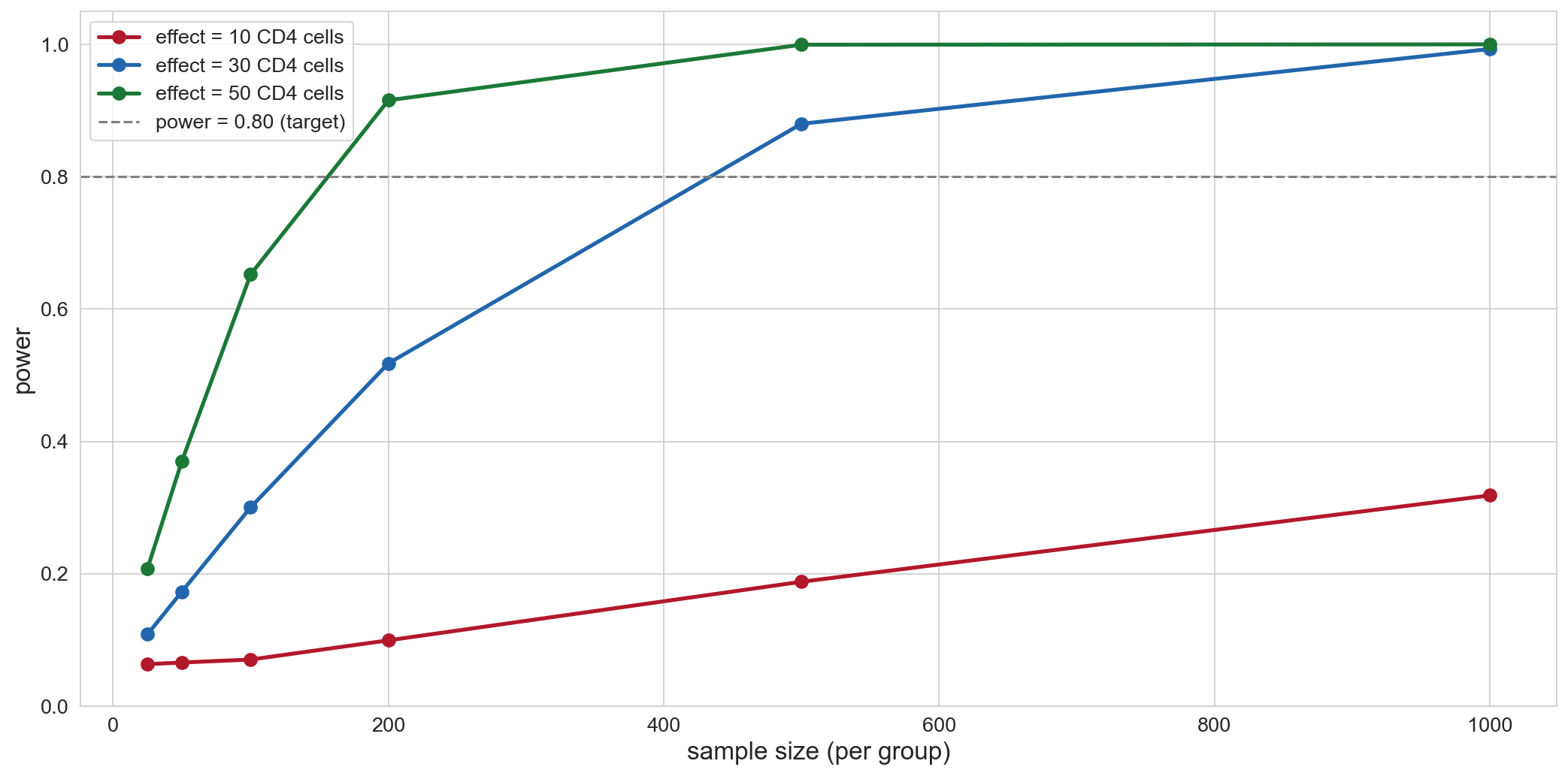
power curves — effect size vs sample size

• large effect (50 CD4): detectable with small samples
• small effect (10 CD4): needs hundreds per group
• gray line = 80% power target

The same picture from before, with our new vocabulary attached. Three curves for three effect sizes plotted against sample size. Find where each crosses the gray 0.80 line — that’s the n you need for that effect. Going from “detect 50-cell effects” to “detect 10-cell effects” pushes required n up by more than 25× — the curves are wildly nonlinear in Δ.

sample size planning — the formula

from statsmodels.stats.power import TTestIndPower
power_analysis = TTestIndPower()

n_needed = power_analysis.solve_power(
    effect_size=0.29,   # Cohen's d = 30 / 105
    power=0.8,
    alpha=0.05
)
# → ~190 per group

Cohen’s \(d = \Delta / \sigma\) — effect in standard-deviation units

(small \(\approx\) 0.2, medium \(\approx\) 0.5, large \(\approx\) 0.8)

The packaged version. Cohen’s d normalizes the effect by the population SD so the answer is unit-free. For ACTG, σ ≈ 105 cells of patient variation, and a 30-cell effect gives d ≈ 0.29 — small-to-medium in Cohen’s convention. To detect that with 80% power at α = 0.05, we need about 190 per group. ACTG 175 actually enrolled over 1,000 per arm — overpowered for the main analysis, which is what you want if you also plan subgroup analyses.

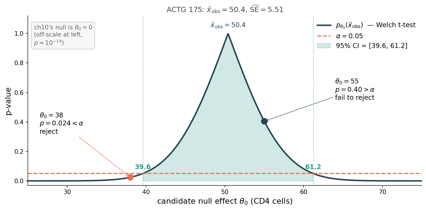
CI/test duality — one curve, two readings

• CI = where the curve sits above \(\alpha\)
• reject = where the curve dips below \(\alpha\)

The duality made visual. Fix the observed data; plot the p-value as a function of the candidate null θ₀. You get one curve, peaked at the observed mean (where p = 1 by definition — the data are perfectly consistent with the null θ₀ = \(\bar x_{\rm obs}\)). Now draw a horizontal line at α = 0.05.

Read the picture two ways. The shaded region — the part of the curve sitting above α — is exactly the 95% CI: [39.6, 61.2]. Any θ₀ where the curve dips below α is a value the test would reject. Two illustrative points: θ₀ = 55 sits inside the CI (p = 0.40, fail to reject); θ₀ = 38 sits just outside (p = 0.024, reject). The CI endpoints are literally where the curve crosses α — that’s the duality.

The chapter’s actual null is θ₀ = 0, far off-scale to the left, with p ≈ 10⁻¹⁹ — way below α, way outside CI. Both readings agree.

Practical takeaway: once you have a CI from Ch 8, you have a “did-this-θ₀-test-reject” oracle for every θ₀ at once. The CI is strictly more informative than any single test. Bootstrap (Ch 8) and permutation (Ch 9) gave the same conclusion not by coincidence — they’re two paths to the same horizontal-line test against this curve.

use tests only when you need a binary decision

binary decision (ship / don’t-ship, approve / reject)

→ hypothesis test is the right tool

every other question — how big is the effect? how uncertain?

→ reach for a CI

most common statistical mistake in industry: using a test when estimation would have answered the actual question

The Wasserman meta-rule, distilled. Hypothesis testing is the right tool when you need to commit to a binary decision: ship/don’t-ship, approve/reject, refer/don’t-refer. For everything else — including the vast majority of analytical questions — a confidence interval gives the entire range of plausible answers and lets the reader decide. The “CI is strictly more informative” point from the duality slide is a special case: when the question is about the parameter’s value rather than a yes/no decision, the CI dominates. Use tests when the decision is genuinely binary; use CIs by default.

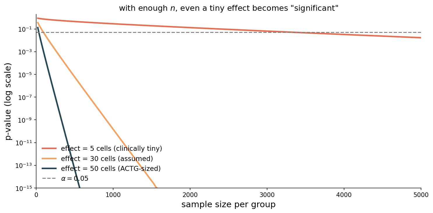
significance ≠ importance

with enough data, anything is “significant”

p-value shrinks as the standard error shrinks (\(\propto 1/\sqrt{n}\))

the effect itself doesn’t have to be large — only nonzero

The failure mode of well-funded studies, visualized. Three real-effect sizes: 5 cells (clinically tiny), 30 cells (the design assumption from earlier in the lecture), 50 cells (the actual ACTG effect). All three lines slope down as n grows — log scale on the y-axis, so each line is geometric decay in p. SE scales like 1/√n; the t-statistic grows as √n; the p-value collapses correspondingly. With n ~ 4000 per arm, even a 5-cell effect — half the size of a coffee-induced blood-pressure bump — crosses α = 0.05. The p-value tells you the effect is unlikely to be zero. It says nothing about whether the effect is large enough to matter.

the blood pressure drug

a clinical trial with 10,000 participants finds:

• p = 0.013 (statistically significant at \(\alpha = 0.05\))
• actual effect: 2 mmHg decrease in systolic BP

for context: a cup of coffee temporarily raises BP by about 5 mmHg

the drug’s effect is real — it’s not zero — but it’s smaller than your morning coffee

Mesas et al., Journal of Hypertension, 2011

The canonical example. The drug works — the p-value confirms the effect is not zero. But the effect is 2 mmHg, while coffee causes a 5 mmHg transient bump. Would you prescribe a daily drug with side effects and cost to achieve less than coffee does temporarily? Statistical significance: not zero. Practical importance: a separate question requiring domain knowledge — what reduction is clinically meaningful, what are the side effects, what alternatives exist.

blood pressure drug: p = 0.013, effect = 2 mmHg, n = 10,000

would you recommend it?

consider:

• costs and side effects
• alternative treatments
• what “clinically meaningful” means

DISCUSSION: Design challenge (5 min). Take a position and defend it; what additional information would change your mind? Prompt: Would you recommend this drug? Process goal: force the distinction between statistical significance and practical importance into a concrete decision. Defensible answers: - “No — 2 mmHg is clinically meaningless. Lifestyle changes (exercise, diet) produce 5-10 mmHg reductions without side effects.” - “It depends — if this is the only option for patients who can’t exercise and are already on other medications, even 2 mmHg might matter at the population level.” - “Need more info — what are the side effects? What’s the baseline blood pressure? What does the drug cost?” If stuck: “Would you take a daily pill to get an effect smaller than your morning coffee?” Key insight: always report effect sizes and CIs alongside p-values.

always report effect sizes

a small p-value tells you: effect is unlikely to be zero

it does not tell you: the effect is large or important

always report:

• effect size
• confidence interval
• p-value

all three together — never p-value alone

The practical takeaway. In any analysis, report all three: effect size (how big?), CI (how uncertain?), p-value (how surprising under the null?). A p-value alone is nearly meaningless without the effect size. Journals increasingly require effect sizes and CIs for this reason. There’s also a darker side to p-value-only reporting, which Ch 11 takes up: when p < 0.05 becomes a publication target, researchers (often unconsciously) p-hack until they cross it. That’s Goodhart’s law applied to scientific evidence.

summary

• Ch 10 = study design: two errors, formula-based test, power analysis
• \(H_1\) is a family — power analysis forces us to pick a specific effect inside it
• Welch’s t-test is the formula-based analog of permutation — solvable for studies you haven’t run yet
• use estimation by default; reach for tests when the decision is binary
• always report effect sizes alongside p-values

Four takeaways. Ch 10 is the prospective complement to Ch 9’s retrospective view — the difference is that we’re now reasoning about studies we haven’t run. The composite-H₁ point is the conceptual hinge: testing doesn’t need an effect size; power does. Welch’s gives us the closed-form null distribution that makes power analysis possible. And the universal practical guideline: report effect size + CI + p-value, every time.

next time

we can test one hypothesis carefully

what happens when you test 20 at once?

Ch 11: multiple testing, Bonferroni correction, false discovery rate, p-hacking

Forward pointer. Today’s framework handles one test perfectly well. But scientists routinely test many hypotheses — 200 NBA players for load-management effects, 20 drug combinations, every feature in a regression. With 20 tests at α = 0.05, you expect one false positive even if nothing is real. Ch 11: Bonferroni, FDR, and the replication crisis.

one-minute feedback

1. what was the most useful thing you learned today?
2. what was the most confusing?

give feedback

Closing ritual. Keep the slide up until the room clears.