Lecture 9: Permutation Tests

MSE 125 — Applied Statistics

Madeleine Udell

Monday, April 27, 2026

the bootstrap says the drug works

but a skeptic asks: how surprised should we be if the drug did nothing at all?

Open with the hook. Last lecture, the bootstrap CI for the ACTG 175 treatment effect was [39.6, 61.3] — entirely above zero. That looks convincing. But the bootstrap measures precision — how much our estimate jiggles from sample to sample. A skeptic wants a different answer: if the drug had NO effect whatsoever, what’s the probability of seeing a gap this large purely by chance? That’s the question the permutation test answers. Same dataset, same trial, different question.

logistics

• HW 2 review sessions: this week
• project meeting with CA: before May 1; sign up! https://stanford-mse-125.github.io/web/project
• quiz 4: Wed Apr 29 — bootstrap + permutation tests (Lec 8-9)
• project proposal: due Fri May 1
• HW 3: due Fri May 8

START RECORDING.

Thirty seconds. Quiz Wednesday covers bootstrap (last lecture) and permutation tests (today). Project proposal is a one-pager due Friday. HW 3 is out — uses both bootstrap and permutation tests.

today

• permutation tests: shuffle labels to simulate “no effect”
• the null distribution: 10,000 permutations map out what chance looks like
• the p-value: how surprised should we be?
• second example: do NBA refs favor the home team? — association vs causation
• one-sided vs two-sided tests — and why the default is two-sided

Five beats. First: the core insight — if the drug does nothing, treatment labels are meaningless, so shuffling them should produce effects that look like ours. Second: do this 10,000 times to build the null distribution. Third: compute the p-value and address the number-one misconception. Fourth: a second dataset — NBA home vs. away personal fouls, testing the folk hypothesis that refs favor home teams. Groups aren’t randomly assigned, so rejecting the null tells us less; and the evidence is marginal here, unlike the overwhelming ACTG case. Fifth: one-sided vs two-sided — and the NBA data shows the verdict flips at α=0.05, which is exactly why direction must be pre-registered. The CI/test connection from Ch 8 gets formalized in Ch 10.

The Lady Tasting Tea — your turn

Rothamsted, 1920s. Muriel Bristol (algae researcher) claims she can taste whether milk went into the cup before or after the tea.

R.A. Fisher’s test: 8 cups, 4 of each kind, in random order — Bristol picks out the 4 “milk first” cups.

your turn. on scrap paper, write M or T for each of positions 1–8. Pick 4 of each — make your best guess at the sequence.

…and the actual sequence:

M · T · M · M · T · T · T · M

show of hands: who got all 4 milk-firsts right?

\(\binom{8}{4} = 70\) arrangements → pure guessing hits the right answer 1 in 70 (~1.4%)

with ~120 of us guessing, we’d expect 1 or 2 winners by luck alone

Bristol got all eight right. that is not luck — it’s a permutation test in miniature.

Fisher (1935) The Design of Experiments; Salsburg (2001) The Lady Tasting Tea.

The origin story for permutation tests — and a live demonstration. Bristol was a serious scientist at Rothamsted (algae researcher) who claimed she could taste the order of milk/tea pouring. Fisher took her seriously and designed the test on the next slide.

Facilitation for the interactive part: 1. On slide 1, read the setup and prompt. Give students 15 seconds to write M/T/M/… picking 4 of each. If they pick 3 or 5 milks, that’s still guessing; don’t police the constraint. 2. Flip to the reveal slide. The sequence M T M M T T T M is just one of the 70 arrangements — the “actual” for today’s demo. You can pick a different sequence if you prefer; change the slide body to match. 3. Ask for a show of hands: who got all 4 milk-firsts correct? There are 70 arrangements; under pure guessing, each student has a 1/70 = 1.4% chance. In a ~120-person class, expect 1-2 hands up; occasionally zero. 4. Land the lesson: Fisher asked “what would guessing look like?” and answered it combinatorially. Bristol got all 8 right — a 1-in-70 event under guessing. That either means she can really tell, or we just witnessed a 1-in-70 coincidence. This is exactly the shape of the reasoning we’re about to apply to a 2,100-patient HIV trial.

if the drug does nothing, labels don’t matter

ACTG 175 — where we left off

treatment_mean = 33.3     # CD4 change, combination therapy
control_mean   = -17.1    # CD4 change, AZT monotherapy

observed_effect = 33.3 - (-17.1)   # = 50.4 CD4 cells

bootstrap 95% CI: [39.6, 61.3] — CI excludes 0, so at the 5% level, the effect is real

so why do a hypothesis test?

• history. p-values (Fisher, 1925) came first; CIs (Neyman, 1937) are the inversion of a test
• generality. tests extend where CIs don’t — counts, orderings, whole distributions (the Lady Tasting Tea)
• language. reject, α, p-value — how science reports evidence

Quick recap of the data — not a recap of concepts, just the numbers we’ll use. Treatment group gained 33 cells on average, control lost 17 (the “control” is AZT monotherapy, not placebo — ethics of 1991 HIV trials). Observed effect 50.4 CD4 cells. Bootstrap CI excludes zero, so the data are already inconsistent with “no effect” at the 5% level — Ch 10 formalizes the link to tests.

So why spend a chapter on hypothesis tests when the CI does the same work? Three honest reasons: (1) History — Fisher’s p-value came a decade before Neyman’s CI. Neyman invented the CI by inverting a test, not the other way around. (2) Generality — the permutation test extends cleanly to settings where a CI isn’t the right shape (the Lady Tasting Tea we just saw is about ordering, not a mean). (3) Language — p-value, reject, α, Type I error are the lingua franca of scientific and industry reporting. You’ll see them in every paper, clinical trial, and A/B test; you need to speak the language. The two frameworks agree on the same evidence — Ch 10 makes the link precise — but the test vocabulary is what you’ll encounter in the wild.

the key insight

if the drug has no effect, each patient’s CD4 change is determined by the patient — not by the treatment label

treatment labels are meaningless

so shuffling them should produce results that look like the real data

but if our observed effect is way larger than anything shuffling produces — the drug works

This is the whole conceptual move. Under the null hypothesis of no effect, which group a patient was in doesn’t matter — their CD4 change would have been the same either way. So if we randomly reassign the labels “treatment” and “control” to the same pool of patients, the fake difference in means should look like just noise. If the real observed difference is much larger than what any shuffling produces, that’s evidence the labels DO matter — the drug has an effect. The logic is airtight: we only need the assumption that under no effect, labels are interchangeable.

observed effect: +50.4 CD4 cells

shuffle treatment/control labels under the null. what difference do you expect?

• A. still about +50
• B. close to 0
• C. could be anything
• D. exactly 0

DISCUSSION: Predict-then-reveal (3 min). Commit to A, B, C, or D; defend to a neighbor; debrief. Process goal: establish the intuition that shuffled effects should be near zero before formalizing the null distribution. Correct answer: B — close to 0 but not exactly 0. The pool of CD4 changes has a grand mean somewhere between the two group means. Randomly splitting into two groups of similar size gives means that are close to the grand mean, so their difference is close to zero. Not exactly zero — sampling variation means each shuffle gives a slightly different split. And not “could be anything” — the law of large numbers keeps shuffled means close to the grand mean. A would only happen if the drug actually works, which is what the null denies. If stuck: “If labels don’t matter, what determines the two group means? Just luck of the draw.” Key insight: Under the null, the expected difference is exactly 0, but any one shuffle gives a small random deviation around 0.

five shuffles

np.random.seed(42)   # so everyone sees the same shuffles

def permutation_diff_of_means(values, n_first):
    shuffled = np.random.permutation(values)
    return shuffled[:n_first].mean() - shuffled[n_first:].mean()

Permutation 1: fake effect = +3.2 CD4 cells
Permutation 2: fake effect = -1.8 CD4 cells
Permutation 3: fake effect = +0.5 CD4 cells
Permutation 4: fake effect = -4.1 CD4 cells
Permutation 5: fake effect = +2.7 CD4 cells

fake effects bounce around zero — observed effect was +50.4

Five shuffles to build intuition before we scale up. The function takes all CD4 changes (ignoring labels), shuffles them, assigns the first n_control to “fake control” and the rest to “fake treatment,” and computes the difference in means. Five random shuffles give values scattered around zero — a few cells positive, a few negative. The largest is about 4 cells. Our observed effect was 50 cells — an order of magnitude larger than what chance produces. Five shuffles aren’t enough for a formal test, but the signal is already clear.

permutation tests: the recipe

1. combine all CD4 changes into one pool (ignore labels)
2. randomly assign \(n_C\) to “control,” the remaining \(n_T\) to “treatment”
3. compute the test statistic on the fake groups
4. repeat many times
5. compare the observed effect to the distribution of fake effects

steps 1-4 build the null distribution

step 5 asks: how extreme is our result?

Name what we just did. Five shuffles made the pattern concrete — now write it down as a portable procedure. Same structure as the bootstrap recipe from last lecture — resample and compute — but the resampling mechanism is different. Bootstrap resamples within each group with replacement. Permutation shuffles labels across groups without replacement. Bootstrap measures precision of an estimate. Permutation measures whether the effect could be zero. Students should memorize both recipes and the distinction. Next, we name the two pieces the recipe refers to (null hypothesis, test statistic) and then scale up from five shuffles to ten thousand.

now we need vocabulary

null hypothesis

the default claim a test tries to disprove

here: “the drug has no effect on CD4 count”

test statistic

the number we compute from the data to measure the effect

here: difference in group means

Name the two pieces before proceeding. The null hypothesis is the claim we’re trying to disprove — here, the drug has no effect. It’s “null” in the sense of “nothing” — nothing is going on beyond random noise. The test statistic is what we compute to measure the effect. For comparing two group means, the natural test statistic is their difference. These are informal definitions — Chapter 10 formalizes with H_0, H_1, alpha, and the full framework. For today, these two concepts are enough.

the permutation test — definition

permutation test

a hypothesis test that builds the null distribution by shuffling group labels and recomputing the test statistic

null distribution

the distribution of the test statistic when the null hypothesis is true

key assumption: labels are exchangeable under the null

Formal definition. A permutation test simulates what would happen if the null hypothesis were true by shuffling group labels. Each shuffle produces one draw from the null distribution — the distribution of the test statistic when the null is true. If the observed test statistic falls far into the tail of the null distribution, we have evidence against the null. The assumption is exchangeability: swapping labels doesn’t change the joint distribution of the data under the null. Random assignment guarantees this — if the drug has no effect, it doesn’t matter which group a patient was assigned to.

from the null hypothesis to the null distribution

• null hypothesis — a claim about the world: “the drug has no effect”
• null distribution — the distribution of the test statistic if that claim were true

the permutation test builds the second from the first — by shuffling

Quick terminology guardrail — students routinely conflate these two. The null HYPOTHESIS is a claim about the world (often “no effect”, “no difference”). The null DISTRIBUTION is the sampling distribution of the test statistic you’d see IF that claim were true. Permutation is a machine that turns the hypothesis into the distribution: every shuffle is one draw from the null distribution, because under the null the labels carry no information. Flag this distinction now; it’ll come back in Ch 10 when we formalize \(H_0\), \(H_1\), \(\alpha\).

why does shuffling simulate from the null distribution?

ACTG 175 patients were randomly assigned to treatment groups

exchangeability

swapping labels does not change the joint distribution of the data under the null

random assignment guarantees exchangeability:

• under the null, the drug has no effect on outcomes
• outcomes don’t depend on labels
• shuffled data is just as plausible as the original

This is the logical foundation. Random assignment means every patient had an equal chance of being in treatment or control, determined by a coin flip (or its clinical-trial equivalent). Under the null hypothesis of no effect, the CD4 outcomes are the same regardless of which group a patient was in. That means any permutation of the labels is equally likely to have been the actual assignment. This property — exchangeability — is what makes the permutation test valid. Without it (as we’ll see in the Airbnb example), the test still detects differences between groups, but the interpretation changes from causal to associational.

building the null distribution

n_perms = 10_000
perm_effects = np.array([
    permutation_diff_of_means(all_cd4, n_T)
    for _ in range(n_perms)
])

Null distribution summary:
  Mean: +0.01
  SD:   5.94
  Min:  -22.40
  Max:  +21.70

tightly centered around zero — SD is about 6 cells

our observed effect of 50 cells is roughly \(50 / 6 \approx\) 8 SD away

Scale up from five to 10,000 permutations. The null distribution is centered at zero (as expected — shuffling preserves the grand mean) with a standard deviation of about 6 CD4 cells. The most extreme fake effect across all 10,000 permutations is about 22 cells. Our observed effect of 50 cells is more than 8 standard deviations above the center of the null distribution. In a normal distribution, 8 SD is essentially impossible. Next slide: the picture.

the null distribution — visualized

where do you expect the observed +50.4 to land?

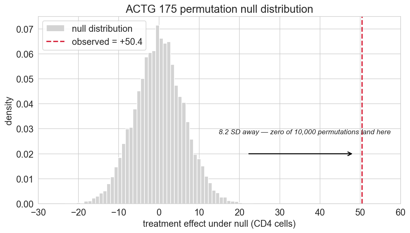
not even close to what random shuffling produces

Predict-then-reveal: before loading the histogram, ask students to sketch (or point on their neighbor’s paper) where they expect the observed +50.4 to sit relative to a null built from 10,000 shuffles. 15 seconds. Then reveal the picture. Null clusters tightly around zero, spans roughly -20 to +20. The red dashed line at +50 sits far to the right — completely separated. No permutation came close. If your sketch put the observed near the edge of the null, the real gap is bigger. Overwhelming evidence against the null. The drug works.

the p-value

p-value

the probability of observing a result at least as extreme as what you got, assuming the null hypothesis is true

the p-value answers: if there were truly no effect, how often would we see something this extreme?

Now we can name the number. The p-value is the fraction of permutations that produced a test statistic at least as extreme as the observed one. “At least as extreme” means in either direction — we’ll use a two-sided test. The p-value is a probability under the null. It is NOT the probability that the null is true — that’s the most common misconception, addressed two slides from now.

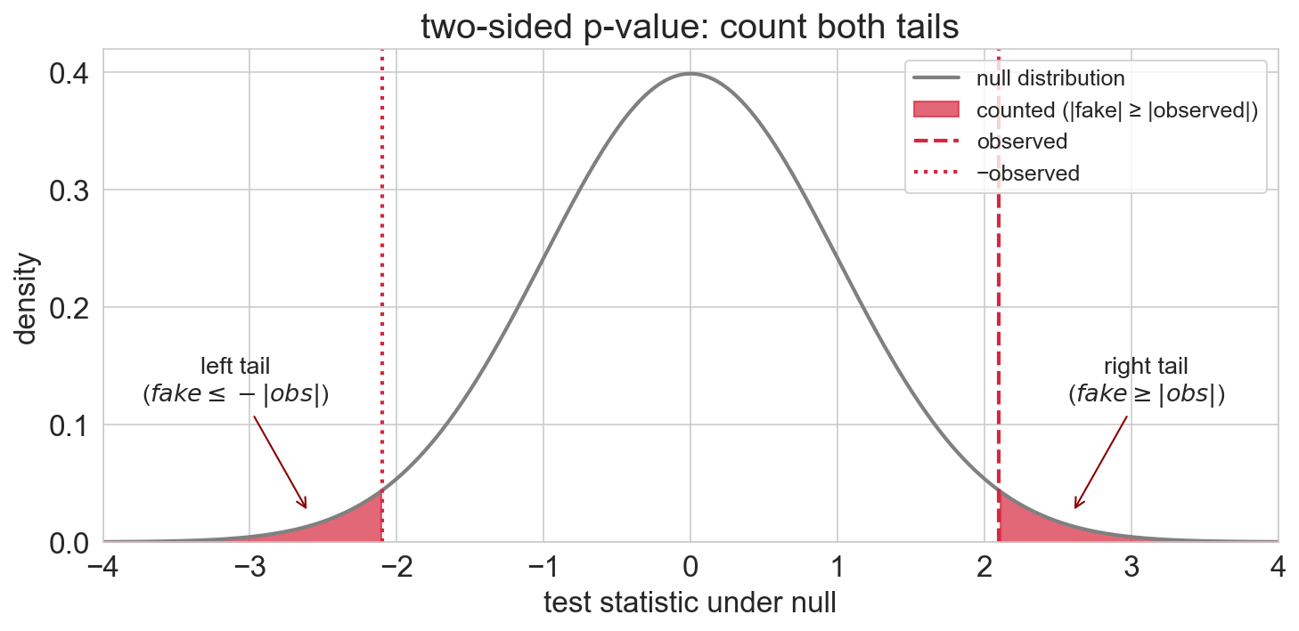
computing the p-value

two-sided: count permutations where \(|\text{fake effect}| \geq |\text{observed effect}|\) — extreme in either direction

n_extreme = np.sum(np.abs(perm_effects) >= np.abs(observed_effect))
p_value = (n_extreme + 1) / (n_perms + 1)

Permutations with |effect| >= |50.4|: 0
p-value: 0.0001

Two-sided counting rule: permutations whose absolute effect is at least as large as 50.4, in either direction — a drug that dramatically helped or dramatically hurt would both count. Zero of 10,000 permutations reached it. Report p ≈ 0.0001.

Why \(+1/+1\)? The identity permutation is also a permutation, and under the null it’s equidistributed with every other. Counting the observed data as one of the \(m+1\) permutations prevents \(p = 0\) exactly, which no finite simulation can earn. So \(\frac{0 + 1}{10{,}000 + 1} \approx 0.0001\) is the simulation floor. The estimator is conservative — its expected value under the null is at least the true tail probability, so false positives are still controlled at the nominal level (Phipson & Smyth 2010). Say one line if asked (“we count the observed data as one extra permutation to avoid reporting p = 0 from a finite simulation”); don’t read the whole justification unless asked.

overwhelming evidence

ACTG 175: \(p \approx 10^{-4}\) — the observed effect lives in a place the null never visits

hold onto this number — we’ll revisit what “overwhelming” feels like once we see data where the evidence is much thinner

Brief setup for the contrast we’ll hit in the NBA example. A p-value of 10^-4 is not just “small,” it’s “the observed effect is in a region the null distribution literally doesn’t reach across 10,000 draws.” This is what overwhelming evidence looks like. In a few slides we’ll do the same test on NBA personal fouls and get p ≈ 0.05 — same mechanics, very different verdict. The contrast is the point: a p-value is a continuous measure, and “p ≈ 10^-4” and “p ≈ 0.05” license radically different claims.

what the p-value is

a probability statement about the data, given the null

• conditions on the null — if no effect, the data would be unlikely
• continuous evidence, not a verdict — \(p \approx 10^{-4}\) far stronger than \(p \approx 0.04\)
• observed data only — replication, mechanism, priors not in the formula

Pin down what the p-value IS before listing what it isn’t. The skeptic’s misconception in the next slide is one of the IS NOTs — framing IS first lets students recognize the shape of the error. Three implications follow from “P(data | H_0)”: (1) it conditions on the null, so a small p-value means “data would be unlikely IF no effect,” (2) continuous — p ≈ 10^-4 and p ≈ 0.04 license radically different claims even though both clear 0.05, (3) the formula doesn’t know about replication, mechanism, or prior plausibility. Keep this slide tight — the discussion is where the learning lands.

a skeptic says:

“a p-value of 0.0001 means there’s only a 0.01% chance the drug doesn’t work”

is the skeptic right?

DISCUSSION: Think-pair-share (4 min total). Think and jot; pair and compare; debrief. Hint to deliver verbally if students get stuck: “what does the p-value condition on?” Process goal: this is the single most important misconception in the entire course. Students must articulate the error in the skeptic’s reasoning before we reveal the correction. Correct answer: the skeptic is wrong. The p-value is the probability of data this extreme given the null is true — not the probability the null is true given the data. The direction of the conditional matters enormously. P(extreme data | null true) is what we computed. P(null true | extreme data) is what the skeptic claims, which would require Bayes’ theorem and a prior probability on the null hypothesis. If stuck: “Analogy: P(it’s raining | I have an umbrella) is not the same as P(I have an umbrella | it’s raining). The order of the conditional matters.” Key insight: The p-value lives in a world where the null IS true and asks how surprising the data are. It does not tell you the probability that the null is true.

three traps

1. NOT the probability \(H_0\) is true — the skeptic’s flipped conditional

2. NOT the probability the result will replicate

3. p = 0.049 and p = 0.051 are not meaningfully different — the 0.05 threshold is a convention

a p-value is a continuous measure of evidence, not a binary verdict

Consolidate the IS NOT story into the same three-trap callout the chapter uses (Ch9 “Three traps”). Trap 1 — flipped conditional — is exactly the skeptic misconception we just resolved in discussion; this slide pins it as item 1 so students leave with one bundled summary, not a scattered two + one. Trap 2 — replication is a separate question; one small p-value doesn’t guarantee the next trial finds the same thing. Trap 3 — the 0.05 threshold is administrative, not scientific, so treating 0.049 and 0.051 as categorically different is a category error. Chapter 10 formalizes the framework with explicit significance levels; for now, the p-value is a continuous measure of surprise.

do refs favor the home team?

folk hypothesis: home teams get called for fewer fouls

same machinery, different interpretation

Transition into the NBA example. Bridge line under the tagline flags the pivot: the shuffle-and-recompute procedure is identical to ACTG, but the conclusions it licenses change completely because nobody randomized games to home vs away. Moskowitz and Wertheim’s Scorecasting (2011) made the popular case that referee bias — not rest, not crowd, not familiarity — explains most of home-court advantage. Their evidence: systematic pro-home bias in called strikes in baseball, stoppage time in soccer, and foul calls in basketball. If they’re right, one place it should show up loudest is in personal foul counts: home teams should be called for fewer of them than their visiting opponents. Three NBA regular seasons give us the data to test it.

NBA personal fouls — the data

# player-level logs -> team-game foul totals
team_game = (logs.groupby(['GAME_ID', 'TEAM_ABBREVIATION', 'MATCHUP'],
                          as_index=False)['PF'].sum())
team_game['home'] = team_game['MATCHUP'].str.contains('vs.')

home_pf = team_game[team_game['home']]['PF'].values
away_pf = team_game[~team_game['home']]['PF'].values
obs_diff_nba = home_pf.mean() - away_pf.mean()

home:  19.36 fouls per game   (n = 3,690 team-games)
away:  19.54 fouls per game   (n = 3,690)
observed gap:   -0.18 fouls per game

Same pipeline we’d build for any NBA question: aggregate player-level rows to team-game totals by summing PF (personal fouls) within each (game, team) pair, then label each team-game as home or away from the MATCHUP string (“vs.” = home, “@” = away). Home teams are called for about 0.18 fewer fouls per game than away teams. That is small against a typical 19-foul game — but the question sharpens when we ask if it’s distinguishable from chance across thousands of team-games.

same null, different interpretation

key difference from ACTG 175: no random assignment here

teams play each opponent home and away — schedule is fixed, not randomized

ACTG 175: “the drug has no effect” — labels exchangeable by random assignment

NBA: “home and away foul counts come from the same distribution”

same null, same permutation mechanics (shuffle labels, recompute)

but rejecting the null only tells us the groups differ — not why

Critically: NOBODY randomized games to home vs. away. The schedule is fixed by the league. Pause here to contrast with ACTG 175, where a coin flip decided each patient’s group. The null hypothesis has the same form: two groups, same distribution. Shuffling is still valid under that null because the label is uninformative about the outcome. What changes is what rejection licenses. In ACTG, rejection + randomization = the drug caused the effect. In NBA, rejection = the home group differs from the away group — full stop. “Referees favor the home team” is one possible story, but being the home team is bundled with rest, travel, crowd, familiarity, scheduling — any of those could produce the gap. The test can’t decompose which.

permutation test finds: home teams get fewer foul calls

• can we conclude referee bias?
• if not — name three alternative mechanisms confounded with home/away

DISCUSSION: Think-pair-share (4 min). Think-pair-share; debrief by collecting explanations on the board. Prompt: Can we conclude referee bias from the NBA permutation test? Process goal: reinforce association vs. causation; students should generate confounders themselves before we rule out “ref bias” as the only story. Correct answer: No — no random assignment means no causal claim. Referee bias is one possibility but not the only one. Alternative mechanisms students should reach: - fatigue and travel: the visiting team has almost always traveled more recently; tired defenders reach in instead of sliding their feet, and reaching fouls get called - scheduling: back-to-backs (two games on consecutive nights) hit the visiting side of a given date more often over a season; compounds fatigue - defensive style: a team may play more (or less) aggressively at home — crowd pressure pushes both ways - familiarity: home team knows its own sightlines, rim stiffness, sideline location; visitors misposition - referee bias: the hypothesis we started with Closest thing to a natural experiment: the 2020 “bubble” playoffs in Orlando — every game on a neutral court with no fans. The permutation test detects the gap but cannot decompose which mechanism produces it; that requires different comparisons. If stuck: “If two teams played on Mars with no fans, would home teams still get called for fewer fouls? Which mechanisms would survive?”

NBA permutation — shuffle labels, recompute

all_pf = np.concatenate([home_pf, away_pf])
n_home = len(home_pf)

perm_diffs = np.array([
    permutation_diff_of_means(all_pf, n_home)
    for _ in range(10_000)
])

n_extreme = np.sum(np.abs(perm_diffs) >= np.abs(obs_diff_nba))
p_value = (n_extreme + 1) / (len(perm_diffs) + 1)

print(f"permutation p-value (two-sided): {p_value:.4f}")

permutation p-value (two-sided): 0.0539

Same machinery as ACTG — pool all foul counts, shuffle, recompute the home-minus-away gap. Ten thousand shuffles. Count permutations whose absolute fake gap is at least as large as the observed 0.18, add the +1/+1 correction, divide. p ≈ 0.054. Next slide: the picture.

NBA fouls — null distribution

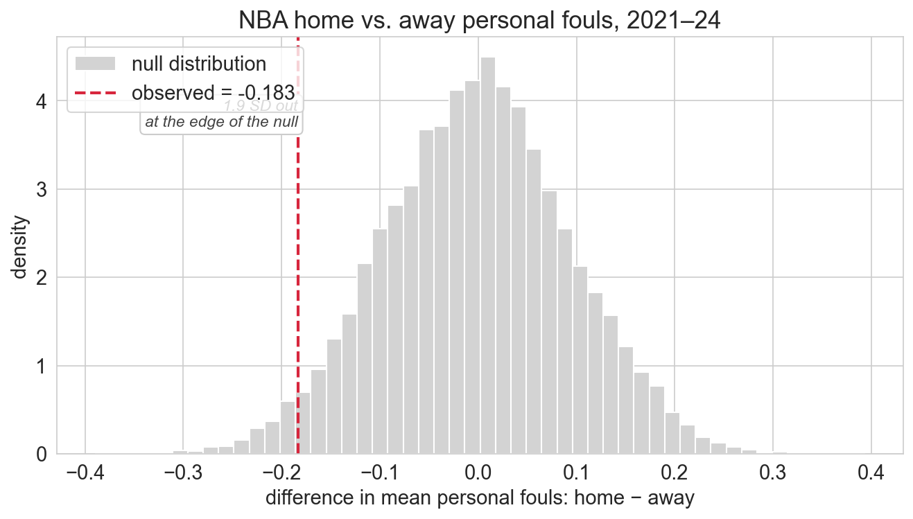
observed gap sits at the edge of the null — not outside it

NBA:  ~540 / 10,000 permutations at least as extreme
ACTG:     0 / 10,000

marginal evidence — contrast with ACTG’s \(p \approx 10^{-4}\)

The histogram of the 10,000 fake gaps. Null sits tightly around zero — chance alone produces gaps up to about ±0.3 fouls per game. The observed −0.18 is at the EDGE of the null, not outside it. About 5% of permutations produce something at least as extreme. Very different picture from ACTG, where zero of 10,000 permutations reached the observed effect. Here, about 540 of 10,000 do. Read honestly: the data are marginally suggestive of a home-away difference in foul calls, not decisive. The contrast with ACTG (overwhelming) vs NBA fouls (marginal) is the point — both would be called “statistically significant” by the 0.05 rule-of-thumb, but they support very different statements. Report the number, not a yes/no.

what if the question were narrower?

“home teams get called for fewer fouls”

not “they get called for different fouls”

one-sided vs two-sided

two-sided vs one-sided tests

two-sided — count fake effects at least as extreme as \(|\text{obs}|\) in either direction

one-sided — count only one tail (direction chosen in advance)

Bridge to the one-sided idea. The NBA question we just ran was two-sided — “do the groups differ in either direction” — because we counted fake gaps extreme on both sides. But the folk hypothesis that motivated the analysis was directional: home teams are called for FEWER fouls. That’s one-sided. We only count fake gaps at least as negative as the observed one.

The picture pairs the two definitions visually: same null distribution on both panels, same observed statistic. Left panel shades both tails beyond ±observed — two-sided, p ≈ 0.054. Right panel shades only the lower tail (the pre-registered direction: home − away < 0) — one-sided, p ≈ 0.029. Same null, different counting rule, different verdict at α=0.05. “Extreme” has a precise meaning that depends on the question.

Under a symmetric null, the one-sided p-value is roughly half the two-sided — “roughly” because Monte Carlo noise and the +1/+1 estimator treat the discrete atoms at ±|obs| slightly asymmetrically. In our actual NBA run, 2 × 0.0288 = 0.0576, not 0.0539 exactly. The approximate 2× relationship is the point — formalized on the next slide.

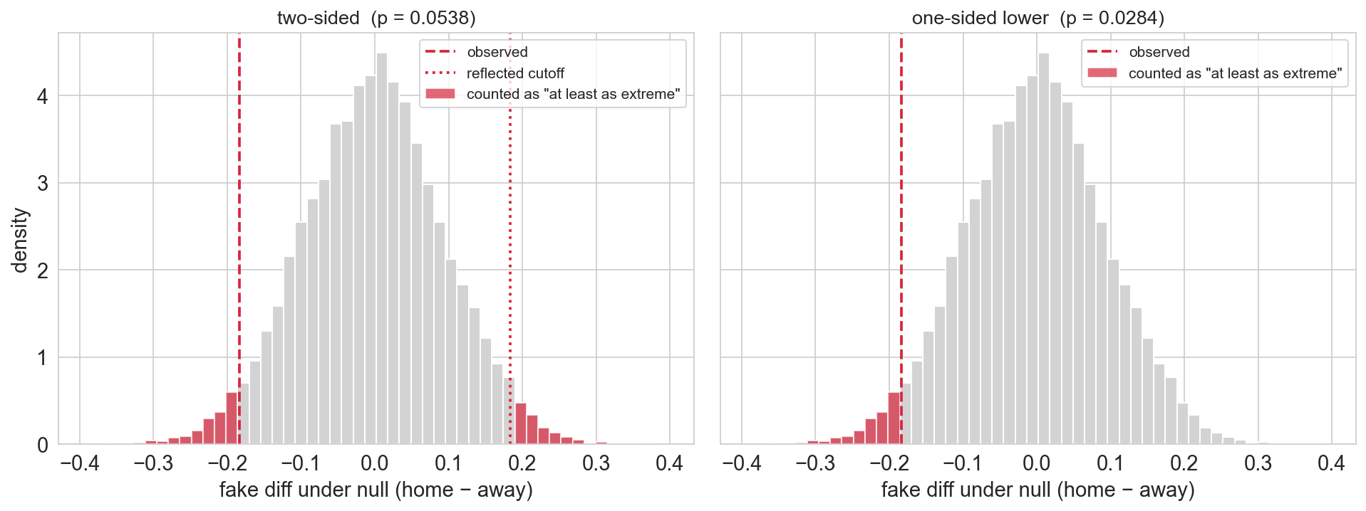
the verdict flips

same data. same null distribution. same observed statistic.

# two-sided: |fake| >= |obs|  — either direction
two_sided = (np.sum(np.abs(perm_diffs) >= np.abs(obs_diff_nba)) + 1) / (len(perm_diffs) + 1)

# one-sided lower: fake <= obs  — pre-registered: home − away < 0
one_sided = (np.sum(perm_diffs <= obs_diff_nba) + 1) / (len(perm_diffs) + 1)

Two-sided p-value:   0.0539    →  FAIL to reject at α = 0.05
One-sided p-value:   0.0288    →  REJECT at α = 0.05

under a symmetric null: two-sided p ≈ 2 × one-sided p — half the tail, half the p-value

the analytic choice — not the data — drives the conclusion — direction must be chosen before seeing the data

This is THE punchline of the one-sided section, and the big upgrade from the old scoring example (where both p-values were at the simulation floor, so the factor-of-two never did anything visible). Here, on real data, the two-sided test fails to reject and the one-sided test rejects. The analyst’s choice of test, not the numbers in the spreadsheet, determines the verdict. That’s why pre-registration matters: if a researcher looks at the data, sees home foul counts were lower, and then declares “one-sided,” they’ve effectively run two tests and doubled their false-positive rate. Post-hoc one-sided = inflated Type I error. Emphasize this slide heavily — students usually don’t feel the factor of two until they see it move the verdict.

The 2× relation is approximate, not exact: if a student does the arithmetic and asks “but 2 × 0.0288 = 0.0576, not 0.0539”, the answer is that the null is discrete and the +1/+1 estimator isn’t symmetric about zero — Monte Carlo rounding. The approximate 2× relationship is the point; the flip is real.

prefer two-sided by default

if you’re not sure, use two-sided — the honest default

a one-sided test is justified only when:

• effects in the other direction are logically impossible or irrelevant
• the direction was chosen before seeing the data

picking the tail post-hoc = effectively running two one-sided tests, each at \(\alpha = 0.05\)

the rate of falsely rejecting a true null jumps from \(\alpha = 0.05\) to \(\approx 0.10\)

Ch 10 formalizes this as the Type I error rate.

The rule: default to two-sided. One-sided is rare in practice — reserve it for contract compliance, tamper detection, or regulatory settings where the other direction is genuinely uninteresting. The Type I error point is the one students most often get wrong: if you look at the data, see that the effect went one way, and then declare “one-sided,” you’ve done two tests (or equivalently, you’ve doubled your false-positive rate). The direction must be pre-registered. We’ll name this false-positive rate formally as the Type I error rate in Chapter 10 — today just plant the idea. Bring this back to the reproducibility crisis — this is one of the small mechanisms that contributes to it.

a high-profile example: Deflategate

Deflategate — a one-sided story

halftime, 2015 AFC Championship. officials measure the game balls.

Patriots’ balls: below the legal minimum. Colts’ balls: fine.

cooling explains some drop — same field, same weather, same physics.

so why did the Pats drop more?

the accusation was directional: Pats dropped more than Colts.

a Pats ball that dropped less → exoneration, not cheating.

only one direction counts as damaging → one-sided test

The cleanest pedagogical example of a one-sided test. Story in order: halftime of the 2015 AFC Championship; officials measure the game balls. Patriots’ balls are below the legal minimum; Colts’ balls are fine (same field, same weather). Cooling physics says both should have lost pressure at the same rate — so the question becomes: why did the Patriots’ balls lose more? That’s the NFL’s accusation — directional. Crucial: a Patriots ball that lost less than the Colts’ would have exonerated the Pats, not indicted them. Only one direction of the statistic counts as damaging. That asymmetry is exactly what a one-sided test encodes. Keep the story to 45 seconds; the pedagogical shape is the point, not the forensics.

state \(H_0\) in plain language → pick one-sided or two-sided

1. factory — contract sets a minimum widget weight; weekly compliance check
2. school district — math curriculum pilot; keep, roll back, or revise?
3. biotech — new cholesterol drug; team hopes it lowers LDL

DISCUSSION: Think-pair-share (5-6 min). Think and jot — null first, then one-sided vs two-sided; pair and compare; debrief by sharing answers and spotting the trap. Prompt: For each scenario, write the null precisely in plain language, then pick one-sided or two-sided. Process goal: force students to commit to a null phrasing before picking the test. The phrasing matters: “doesn’t increase scores” is a different null from “doesn’t change scores,” and they pick out different tests. Debrief in order — widget first (warm-up, contract clarifies the direction), school next (the null-phrasing point), biotech LAST (the safety trap).

Answers: (1) One-sided. \(H_0\): \(\mu \ge w_{\min}\) (shipment meets the minimum); \(H_1\): \(\mu < w_{\min}\). The contract penalizes only under-weight shipments — over-weight is logically exculpatory, not noteworthy. Same structure as Deflategate. (2) Two-sided. \(H_0\): \(\mu_{\text{new}} = \mu_{\text{old}}\) (no change in scores). The right framing is “no change,” not “no increase”: scores that drop drive the rollback decision, so the test has to be able to detect them. A one-sided “doesn’t increase” null would silently treat a score drop as just another way to fail to find an improvement, discarding evidence the district would act on. THIS is the null-phrasing point. (3) Two-sided — a trap. \(H_0\): \(\mu_{\text{new}} = \mu_{\text{control}}\) (drug doesn’t change LDL). Tempting to go one-sided because the team hopes for a decrease, but a drug that raises LDL is a safety signal and would absolutely change the launch decision. Hoping for a direction ≠ only one direction matters. (Aside if asked about FDA practice: real Phase III efficacy trials sometimes use one-sided tests at α=0.025, which is decision-theoretically equivalent to two-sided at α=0.05 — regulatory convention paired with separate safety monitoring. Not a free halving.)

Meta-lesson to surface in debrief: writing the null precisely tells you which test to use. One-sided is genuinely rare outside contract-compliance or tamper-detection contexts. Reserve it for cases where the other direction is logically irrelevant (not merely undesired), and pre-register the choice before looking at the data.

bootstrap vs permutation — when to use which

	bootstrap	permutation test
question	how precise is my estimate?	is the effect real?
produces	confidence interval	p-value
null hypothesis	not needed	required
key assumption	i.i.d. samples in each group	exchangeability under null
best for	any statistic	comparing groups
resampling	with replacement, within each group	without replacement, shuffling across groups

i.i.d. = independent and identically distributed

both are simulation-based inference: the computer builds the reference distribution; no normality or closed-form formula needed

bootstrap = precision \(\quad\) permutation = significance \(\quad\) use both

The comparison table closes the unit. Two datasets shown (ACTG and NBA), two tools (bootstrap + permutation), one summary. Both are simulation-based and nonparametric, but they answer different questions. Bootstrap resamples within each group with replacement to estimate variability. Permutation shuffles labels across groups without replacement to test for differences. Bootstrap gives you a CI; permutation gives you a p-value. Bootstrap doesn’t need a null; permutation does. Punchline: bootstrap = precision, permutation = significance. Use both on the same data for complementary answers.

A/B testing — same idea, different name

in data analytics, the permutation test between two groups is called A/B testing

• A = control \(\quad\) B = treatment
• used at every tech company: feature rollouts, pricing, ad copy, UX tweaks

the machinery is exactly what we just ran — shuffle labels, recompute, compare

Quick vocabulary slide. A/B testing is the industry term for a two-group permutation test — used at every tech company for feature rollouts, marketing campaigns, pricing experiments. “A” and “B” are just “control” and “treatment” renamed. The tool is the permutation test — same shuffle-and-recompute logic. If students go into tech, they will use this constantly. We’ll see A/B testing come back in Ch 11 when we talk about what happens if you run hundreds of these tests in a row (the multiple-testing problem).

summary

• shuffle → null distribution → p-value — the recipe
• small p-value \(\neq\) small probability the null is true — the #1 misconception
• report the number — \(p \approx 10^{-4}\) (ACTG) and \(p \approx 0.05\) (NBA) are different verdicts, not the same “significant”

one recipe — 8 cups of tea, 2,139 clinical patients, 7,000 NBA games

Three punchlines. (1) The recipe: pool, shuffle, recompute, compare — builds the null distribution and gives a p-value. (2) The misconception: the p-value is P(data | null true), not P(null true | data); students leave this lecture with that correction or not at all. (3) Report the number: \(10^{-4}\) and \(0.05\) are both below 0.05 but license radically different claims. The connections back to exchangeability and bootstrap-vs-permutation have their own dedicated slides earlier in the deck; don’t re-recap them here.

next time

we have the p-value — but what threshold should we use?

• Ch 10: formal hypothesis-testing framework — \(H_0\), \(H_1\), \(\alpha\), Type I/II errors, power
• Ch 11: what happens when you run many tests?
• Ch 18: when a test can license causal claims — designing for causation

Forward pointer. Today we computed a p-value but used it informally — “very small, so the drug works.” Chapter 10 formalizes the framework: significance levels, error types, power. Chapter 11 tackles what happens when you run hundreds of tests (genomics, A/B testing at scale) — the multiple testing problem. Chapter 18 picks back up the thread we left at NBA home-court: how do you design an experiment or a natural experiment that lets you make a causal claim, not just an associational one?

one-minute feedback

1. what was the most useful thing you learned today?
2. what was the most confusing?

give feedback

Closing ritual. Ask students to submit before they leave; keep the slide up until the room clears.