Lecture 8: Bootstrap and the Normal Approximation

MSE 125 — Applied Statistics

Madeleine Udell

Wednesday, April 22, 2026

in the early 1990s, AIDS was the leading killer of Americans aged 25–44

the first drug worked — until it stopped working

what next?

Open with the hook. By the early 1990s the US was a decade into an AIDS crisis, and by 1993–94 AIDS had become the leading cause of death for Americans aged 25–44. The one approved drug, AZT, extended lives but the virus evolved resistance. The NIH launched ACTG 175 to compare combination therapy against AZT alone — with the stakes of setting the standard of care for millions of patients worldwide. Today’s lecture is the tool that let researchers say “yes, combination therapy really is better” rather than “we got lucky with our 2,139 patients.”

logistics

• HW 1: grades almost ready. we’ll trial AI grader + feedback for future assignments
• HW 2: due this Friday 11:59pm
• project proposal: due Fri May 1. sign-up to chat with TAs before then — slots open tomorrow. we’ll post project ideas shortly.

START RECORDING.

Thirty seconds. Quiz next Wednesday covers last lecture and today. HW 3 Friday uses the bootstrap directly — you’ll put a CI on a correlation coefficient. Project proposal also due that Friday, one-pager.

today

• the question: can we trust one number from one trial?
• the bootstrap: resample the data to see what else we might have gotten
• the surprise: the answer looks normal
• the payoff: CLT gives a one-line formula — and warns when it fails

Four beats. First: the clinical-trial setup that motivates everything else. Second: the bootstrap as a resampling recipe — works for any statistic. Third: the surprise moment — the bootstrap distribution of the mean looks suspiciously normal. Fourth: the Central Limit Theorem explains why, which gives us a formula (the normal approximation) — and also tells us exactly when the formula fails, so we know when to reach back for the bootstrap.

ACTG 175 — the trial

• enrolled 1991–1993, published 1996
• NIH AIDS Clinical Trials Group
• 2,139 adults with HIV
• four treatment arms — combination therapy vs AZT alone
• outcome: change in CD4 count at 20 weeks

CD4 = the white blood cells HIV destroys

rising count \Rightarrow immune system recovering

Hammer et al., NEJM 1996

Ground the story in the concrete setup. ACTG 175 was a landmark trial. Four arms but we’ll focus on the simplest contrast: any combination therapy vs AZT monotherapy. The outcome is the change in CD4 count from baseline to 20 weeks. CD4 cells are helper T cells — the immune system’s quarterbacks — and HIV kills them. A rising count means the immune system is bouncing back. A falling count means the patient is losing ground. The NEJM paper was the definitive read-out, and it changed practice overnight.

the data

df = pd.read_csv('ACTG175.csv')
df['cd4_change'] = df['cd420'] - df['cd40']

treatment = df[df['treat'] == 1]   # n_T = 1607
control   = df[df['treat'] == 0]   # n_C =  532

print(treatment['cd4_change'].mean())  # 33.3
print(control['cd4_change'].mean())    # -17.1

observed difference of means = 33.3 - (-17.1) = \mathbf{50.4} CD4 cells

treatment gains ≈ 33 cells — control loses ≈ 17 — AZT alone is failing these patients

Concrete code. Compute cd4_change as the difference between week-20 count and baseline. Split into treatment and control groups, look at the mean change in each, and take the difference. After the raw numerical reveal, pause at the clinical-story fragment: the treatment group gains about 33 cells; the control group loses about 17. Let that land — negative CD4 change is not abstract, it means these patients’ immune systems were losing ground on AZT alone. That’s what made combination therapy matter. The gap — 50 cells in favor of combination therapy — is our observed difference of means. We’ll use n_T = 1607 and n_C = 532 as shorthand for the two group sizes throughout the lecture.

estimation — the game we’ve been playing

estimand, estimator, estimate

• estimand — the fixed-but-unknown population quantity
• estimator — the procedure that maps data to a guess
• estimate — the specific number produced by one dataset

you’ve been playing this game since week 1:

lec	estimand	estimator
4	pop’n mean \mu	sample mean \bar X
5	pop’n coefficients \beta	OLS \hat\beta
7	pop’n accuracy	test-set accuracy

today — estimand \mu_T - \mu_C, estimator \bar X_T - \bar X_C, estimate = \mathbf{50.4} CD4 cells

new question: how precise is the estimate?

Retrospective framing. Since Lec 4, every chapter has computed sample statistics and treated them as answers: the sample mean of Airbnb prices, the OLS bedrooms coefficient, the test-set accuracy on Framingham. Each is an estimator of a fixed-but-unknown population quantity; the specific number is the estimate. Today we finally name the game — estimand / estimator / estimate — and install the vocabulary that Lec 9–12 all build on top of. The ACTG example is the first place we go beyond “here’s the number” to ask “how precise is the number?” That’s the new question, and bootstrap + CLT are the tools.

the population distribution

population distribution \mathcal{X}

the distribution of a single observation drawn from the population

• X_i \sim \mathcal{X} — each outcome is one draw
• parameters: mean \mu, SD \sigma — fixed, unknown
• any shape — skewed, bounded, multimodal

ACTG 175 has two populations, two distributions:

• \mathcal{X}_T — CD4 change across all combination-therapy-eligible adults
• \mathcal{X}_C — CD4 change across all AZT-only patients

the 1607 treatment patients and 532 controls in our trial are samples from \mathcal{X}_T and \mathcal{X}_C

Name the object. \mathcal{X} is the distribution you’d see if you could magically observe the outcome of every eligible patient — not what you saw, which was a sample. Its parameters \mu and \sigma are the estimands we care about. Crucially, \mathcal{X} can be any shape — it does not have to be normal. This is the first of three distributions we’ll meet today: \mathcal{X} (the population distribution), the sampling distribution of \bar X_n in a few slides, and the bootstrap distribution later. Keep them straight — they’re different objects with different roles, and conflating them is the single most common source of confusion about inference.

law of large numbers — plug in the sample

LLN: as n \to \infty, sample statistics converge to population parameters

\bar X_n \;\longrightarrow\; \mu, \qquad s_n \;\longrightarrow\; \sigma

you proved this in MS&E 120 — now we’ll use it

so plug in the sample to estimate \mathcal{X}’s parameters:

\hat\mu = \bar X_n, \qquad \hat\sigma = s_n

ACTG treatment group: \hat\mu_T = \bar X_T = 33.3 CD4 cells — our estimate of \mu_T

• LLN — \bar X_n \to \mu, eventually
• CLT (today) — how fast, and in what shape

The LLN is the foundation: it guarantees that averages converge to population parameters, so the sample mean and sample SD are principled estimators. You saw this in MS&E 120 — today we put it to work. The plug-in move: wherever a formula has an unknown population parameter, substitute the corresponding sample statistic. We’ll do this repeatedly — \sigma in the SE formula becomes s, \mu-center of the sampling distribution becomes \bar X. The LLN is necessary but not sufficient — it tells us \bar X \to \mu but not how fast. The CLT, coming in a few slides, sharpens “gets close” into “approximately normal with width \sigma/\sqrt n.” That rate is what lets us build confidence intervals.

two population means — the estimands

population mean

• the average CD4 change across every HIV-positive adult eligible for the trial
• under a given treatment: one mean under combination therapy, one under AZT alone
• each fixed but unknown — we estimate both from the sample

the difference of the two means is often what we care about

under randomization, that difference reads as the drug’s causal effect

Before we do any analysis, name what we’re after. We have two population means we’d like to know: the average CD4 change under combination therapy across every eligible HIV-positive adult, and the average under AZT alone. Neither exists in the data — they’re Platonic quantities we can only estimate. The difference of these two means is what we often call the “treatment effect”; because ACTG 175 was randomized, that difference reads as the drug’s causal effect on CD4 change. But the statistical object is still a pair of population means — the difference falls out as a linear combination. Chapter 18 formalizes the causal reading.

but the spread is enormous

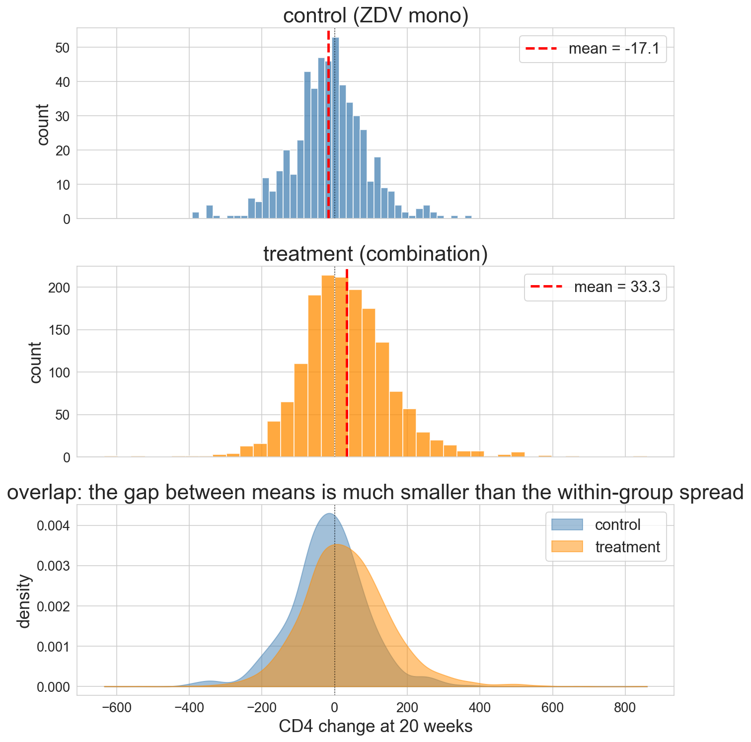
red dashed = group mean

the overlap is bigger than the gap

Show the two histograms side by side — control on the left, treatment on the right. The group means are about 50 cells apart, but the within-group spread is several hundred cells wide. Any individual patient could easily fall in either distribution. Which raises the question: if we re-ran the trial with a different 2,139 patients, would we still see a ~50-cell gap? Or did we get lucky with this particular mix of patients?

what if we only had 50 patients?

for i in range(3):
    sample = np.random.choice(treatment_cd4, size=50, replace=False)
    print(f"sub-trial {i+1}: mean = {sample.mean():.1f}")

sub-trial 1: mean = 48.7
sub-trial 2: mean = 35.8
sub-trial 3: mean = 31.8

three sub-trials, three different answers — sampling variation in action

Drop from the full 1607 treatment patients down to hypothetical sub-trials of 50. Pull three such sub-trials. The three estimates of the treatment-group mean range across a wide band — 49, 36, 32 — purely from which 50 patients happened to get sampled. Same population, same procedure, different luck. This is the whole game. Sample-to-sample variation is why a single observed effect is not enough — we need to know how much the effect would jitter under repeated sampling.

sampling distribution

sampling distribution

the distribution of values a statistic would take if we could repeat the study many times, each time with a fresh sample from the population

the three sub-trials above are three draws from this distribution

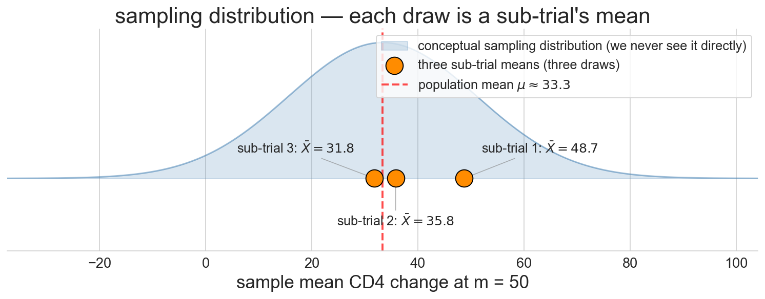
we never see it directly — we have one sample, not many

Name the object the rest of the chapter is trying to approximate. Three orange dots are the three sub-trial means we just computed — each is one draw from the sampling distribution. The faint blue curve is the distribution we’d see if we could draw many more times — but in practice we never get to see this curve directly. The bootstrap is our trick for approximating it. Imagine running the clinical trial 1000 times, each with a fresh random sample of 2139 patients, and collecting 1000 observed treatment effects. The distribution of those 1000 numbers is the sampling distribution of our estimator. It has a mean (close to the true treatment effect), a spread (the standard error), and a shape (often normal — we’ll see why). We never actually do this — we have one trial. The bootstrap is our trick for pretending we can, by resampling the one dataset we have.

the sampling distribution is what we want — but we only have one sample

how do we estimate it?

• A. split our sample into sub-samples and study their variation
• B. run the whole study again — many times
• C. use our one sample cleverly to simulate “alternative studies”
• D. we can’t — there’s no principled way

DISCUSSION: Predict the approach (3 min — 30 sec commit to A/B/C/D, 1 min defend to a neighbor). Prompt: How do we estimate the sampling distribution from a single sample? Process goal: set up the bootstrap as the only principled option by contrast with three tempting alternatives. Correct answer: C — the bootstrap. - A sounds reasonable but gives you the spread of sub-sample means at a smaller sample size — not what you actually face at size 1607. You’d be measuring a different, inflated standard error. - B is impossible in practice: we can’t replay a 1991–1995 trial, and even prospectively it would cost tens of millions and take years. - D is defeatism — a plausible first reaction but wrong. Bradley Efron’s 1979 insight was exactly that there IS a principled way. - C is the chapter’s central technique — the bootstrap: treat our one sample as a stand-in for the population, resample with replacement, and let the jitter across resamples approximate the jitter across studies. If stuck: “We can’t actually re-run the trial. We can’t sub-sample without losing the effective sample size we care about. What’s left?” Next slide opens Block 2 and introduces the bootstrap as the answer.

resample the data you have

the bootstrap — core idea

our one sample is the best picture we have of the population

treat it as if it were the population

draw new samples from it — with replacement

This is the whole conceptual move in three lines. We don’t have the population; we have a sample. Pretend the sample is the population — draw new “samples” from it by picking its rows uniformly at random, with replacement. Each new draw is a plausible alternative version of our dataset. The word “replacement” matters: without it, every resample would be identical to the original (just shuffled). With replacement, some rows appear twice, some don’t appear at all, and we get genuine variation across resamples. That variation is our window into the sampling distribution.

sampling with replacement — a mini trial

trial_patients = ['Alex', 'Jordan', 'Sam', 'Taylor', 'Casey']
resample = np.random.choice(trial_patients, size=5, replace=True)
# example: ['Taylor', 'Casey', 'Jordan', 'Taylor', 'Jordan']

• some patients appear twice
• some are missing

that’s “with replacement”

each resample is a plausible “alternative trial we might have run”

Make “with replacement” concrete with a five-patient mini-trial. Imagine the trial had enrolled only five patients — Alex, Jordan, Sam, Taylor, Casey. The bootstrap pretends this five-person sample is the whole population, and simulates a re-run by drawing five patients uniformly at random with replacement — put each back after drawing. Some patients show up twice; some don’t show up at all. That asymmetry is the source of variation across resamples. Each resample has the same size as the original but different composition. Scale this up from five to 1607 and the mechanic is identical: resample rows with replacement, compute the statistic, repeat.

the bootstrap recipe

1. treat the observed sample as the population
2. draw a resample — same size, with replacement
3. compute the statistic on the resample — mean, median, slope, AUC, …
4. repeat steps 2–3 B times — typically B = 10{,}000
5. the spread of those B values estimates SE; the middle 95% is a 95% CI

works for any statistic — that’s the power

The portable recipe. Memorize the five steps. The statistic in step 3 can be anything — we’ll do the difference in means today, but students will use the same recipe for the median, for regression coefficients (Chapter 12), for classification AUCs, for quantile estimates, for anything that maps a dataset to a number. B is the number of replications and it’s a compute knob — larger is more accurate but slower. The dataset size n is separate — you can’t change that by taking more bootstraps.

what a resample looks like

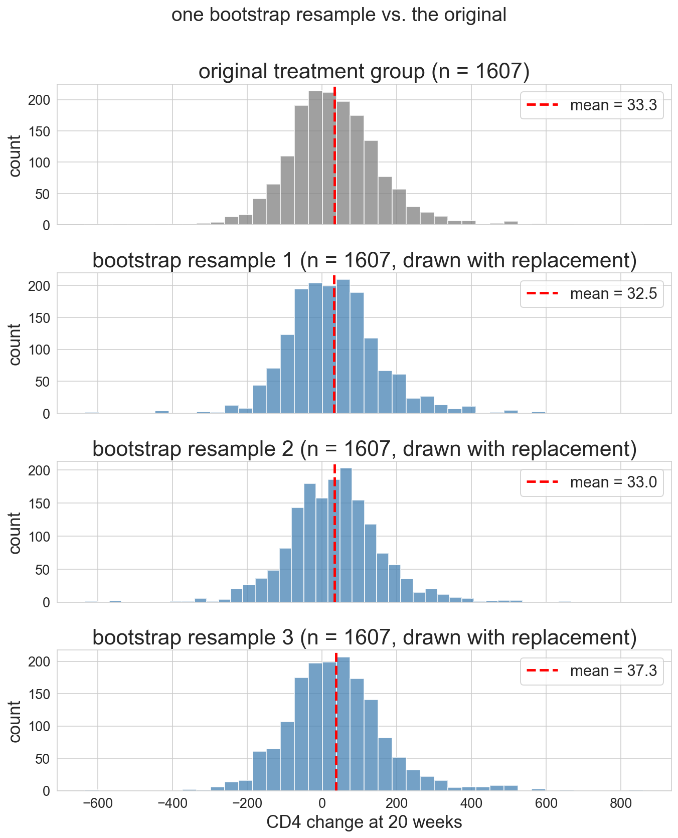
• original on top
• three resamples below
• same size, slightly different composition, slightly different mean

Before we do this 10,000 times and look at the distribution of means, pause on what one resample actually looks like. Top panel: the real treatment group, 1607 patients, mean CD4 change ≈ 33. The three blue panels below: bootstrap resamples, each drawn with replacement from the same 1607 values. The overall shapes are nearly identical — the bootstrap is pretending we re-ran the trial with different luck. The means differ by a cell or two from panel to panel; that’s the sampling-distribution variation we’re trying to measure. When we loop 10,000 times and collect the means, we’ll map out the full distribution of that variation.

bootstrap the difference of means

def bootstrap_diff(t_data, c_data):
    t = np.random.choice(t_data, size=len(t_data), replace=True)
    c = np.random.choice(c_data, size=len(c_data), replace=True)
    return t.mean() - c.mean()

B = 10_000
boot = np.array([bootstrap_diff(treatment_cd4, control_cd4)
                 for _ in range(B)])

np.random.choice(..., replace=True) = one bootstrap resample; list comprehension runs it B times and stacks into an array

B = number of bootstrap replications (here, 10,000) — a separate knob from the dataset size n

boot.mean() = 50.4    ← centered at observed difference
boot.std()  = 5.6     ← ≈ standard error of the estimator

Step through the code. The function resamples both groups independently and returns the difference in their means — one draw from the bootstrap distribution of the estimator. Loop that 10,000 times, collect the results into an array. The mean of that array matches the observed difference; the SD of that array is what we care about — it’s our estimate of the standard error of the estimator. This is the whole point of bootstrapping: we never derived an SE formula, we just simulated.

the bootstrap distribution

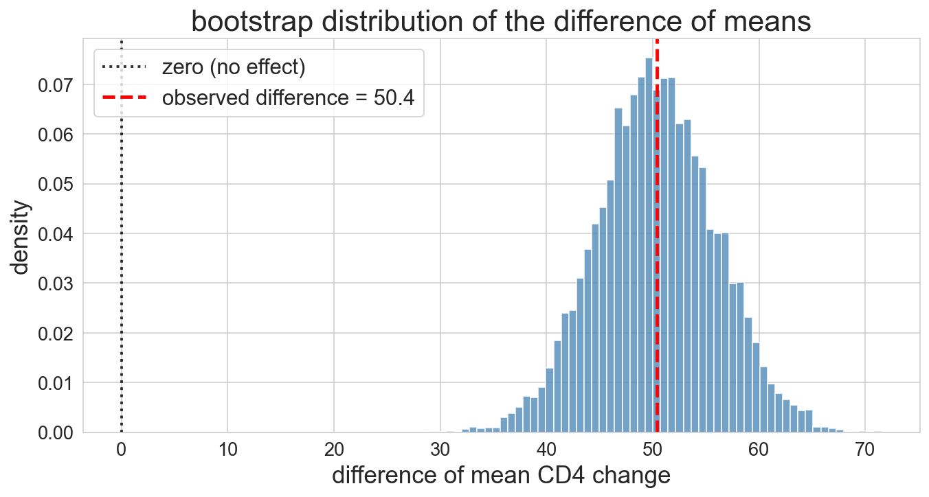
10,000 resamples mapping out the shape of plausible values

our third distribution today — after \mathcal{X} and the sampling distribution of \bar X_n

Visualize the bootstrap distribution as a histogram. The x-axis is “plausible treatment effect in CD4 cells”; the y-axis is frequency across 10,000 resamples. The distribution is clearly centered near 50 and the tails fall off smoothly. Name this explicitly as the third distribution of the lecture: we have \mathcal{X} (the population distribution — what we wish we knew), the sampling distribution of \bar X_n (the distribution of the estimator across repeated studies — what we’d see if we could re-run the trial), and now the bootstrap distribution (the empirical approximation to the sampling distribution — what we actually see). The key claim: because our sample approximates \mathcal{X}, the bootstrap distribution approximates the sampling distribution. Remind students: this is approximate — we haven’t actually re-run the trial 10,000 times, we’ve just resampled the one trial we have. But the shape tells us what plausible answers look like given what we know.

today’s estimand, estimator, estimate

• estimand — \mu_T - \mu_C (population difference of CD4 means)
• estimator — \bar X_T - \bar X_C (difference of sample means)
• estimate — 50.4 CD4 cells (one number from one dataset)

the estimate changes every time you draw a new sample

the estimand stays fixed

the bootstrap just gave us 10,000 estimates — mapping out that variation

Callback to the estimation block from the top of the lecture. The vocabulary is already installed — this slide reinforces with ACTG-specific values. On your flashcards: \mu_T - \mu_C for the estimand, \bar X_T - \bar X_C for the estimator, 50.4 for the estimate. The estimand is fixed; the estimate changes every time we draw a new sample. The bootstrap distribution is the distribution of estimates under resampling — we just computed 10,000 of them, and the spread of that distribution is the standard error of the estimator.

confidence interval — percentile method

95% confidence interval

intuition: a range of plausible values for the estimand

formal: built by a procedure where 95% of intervals contain the estimand across repeated studies

percentile method: the 2.5th to 97.5th percentile of the bootstrap distribution

⚠ not “estimand has a 95% chance of being in [a, b]” — estimand is fixed, CI varies across studies

Two readings of “95% confidence interval” that must not be conflated. The intuition is the practical one — the CI shows a range the estimand is plausibly in. The formal statement is a coverage guarantee over hypothetical repeated trials — across many possible studies, 95% of the intervals built this way would contain the truth. Both readings are useful; neither is “the estimand has a 95% probability of being in [a,b]” — the estimand is fixed, the interval is what varies. Percentile method: sort the 10,000 bootstrap values, take the 250th and 9750th, done. Works well when the bootstrap distribution is roughly symmetric.

• bootstrap mean ≈ 50
• bootstrap SD ≈ 5.6

Q: does the 95% CI include zero?

what would it mean for the drug if the CI did include zero?

DISCUSSION: Predict-then-reveal (3 min — 1 min predict yes/no and say why, then debrief). Debrief hint to deliver verbally: “what’s the rough CI width? ≈ ±2 SD.” Prompt: Does the 95% CI include zero? Process goal: check the rough-CI heuristic (point estimate ± 2 SE) before we reveal the exact percentile CI. Correct answer: no — 50 ± 2·5.6 = [39, 61], well above zero. If the CI did include zero, we could not rule out “no effect” — the trial would be inconclusive about whether combination therapy beats AZT at all. If stuck: “50 is how many SDs above zero? Is that deep into the tail?” Key insight: A CI that excludes zero is the lightweight version of “the effect is statistically significant.” A CI that includes zero is the lightweight version of “the evidence can’t rule out no effect.” We’ll formalize both readings in Ch 9 (permutation) and Ch 10 (hypothesis testing).

and the CI is…

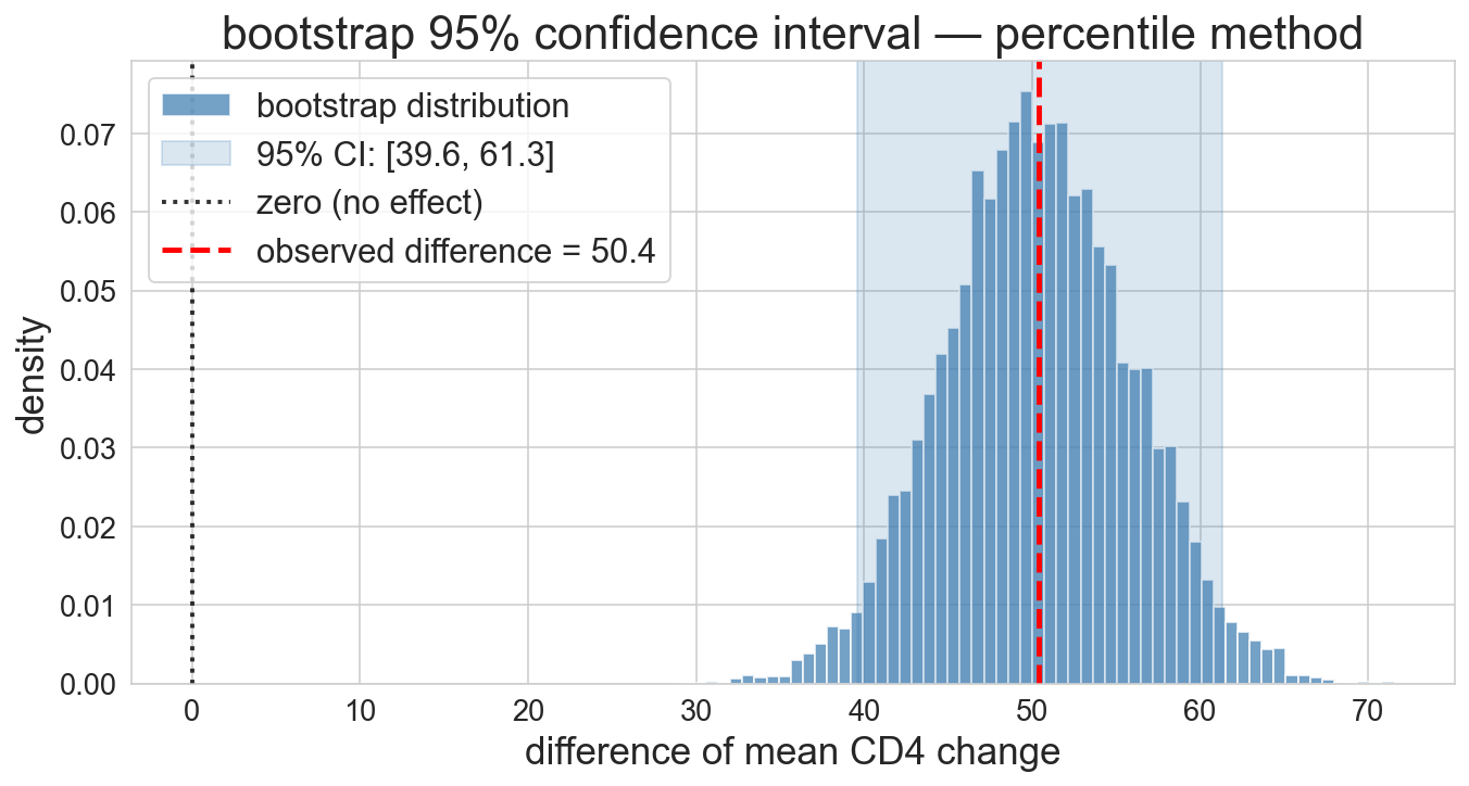
95% CI: [39.6, 61.3]

entirely above zero — the drug really works

Reveal. The CI is [39.7, 61.2]. Nowhere near zero. Combination therapy is genuinely better than AZT monotherapy — the bootstrap gives us quantified uncertainty that still confidently excludes “no effect.” Because ACTG 175 was randomized, the causal reading is licensed: the treatment causes the improvement, not just correlates with it. This result changed practice when published in 1996.

what a CI does and doesn’t cover

does: sampling uncertainty — different patients showing up

doesn’t: systematic shifts — seasonality, a new competitor, a marketing campaign mid-trial

before trusting a CI for a decision, ask: is the uncertainty that matters the kind the bootstrap captures?

Before we move on to why the bootstrap distribution looks normal, pause on what the CI is actually covering. A 95% CI quantifies sampling uncertainty — the scatter we’d see if we re-ran the trial with different patients drawn from the same population. It does NOT cover systematic shifts in the system. Use A/B-test-adjacent examples that’ll resonate with the modal MSE student in 2026: seasonality (holiday checkout behavior is different), a new competitor shipping mid-experiment, a marketing campaign launching halfway through. Resampling rows of a dataset cannot simulate the world changing. The CI tells you about noise around a fixed world, not about whether the world itself might shift. This foreshadows the D4 capstone on the new checkout flow. Chapter 16 on backtesting returns to this point when models trained on historical data meet changed conditions.

it looks normal

the bootstrap distribution looks… bell-shaped?

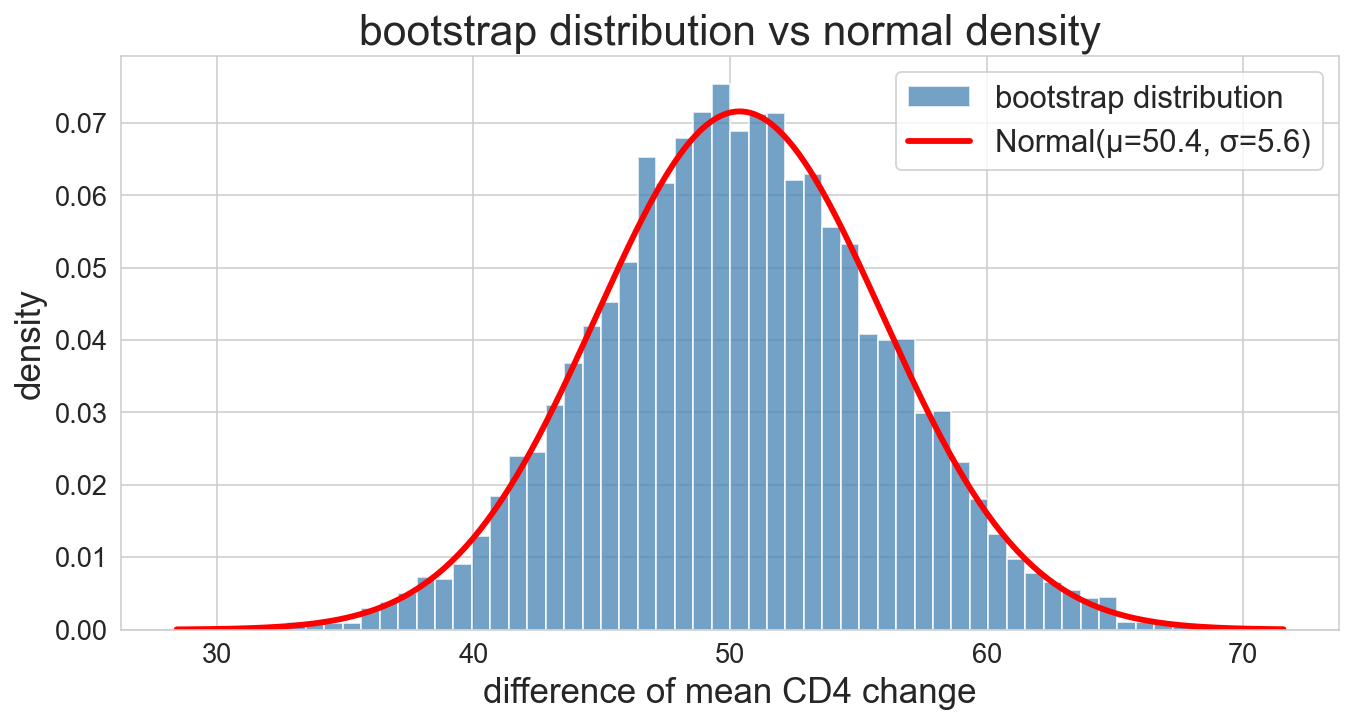
red curve = Normal(μ, σ) with bootstrap mean and SD — nearly perfect fit

Overlay a normal density on top of the bootstrap histogram. The fit is so good that the histogram and the curve are almost indistinguishable. This is the surprise moment of the chapter: we never assumed normality anywhere. CD4 changes are messy patient outcomes. The treatment effect is a difference of means. And yet the bootstrap distribution of that difference is textbook normal. Why?

Central Limit Theorem — informal

if you average many independent draws from a population distribution \mathcal{X}, the result is approximately normal — for large enough sample size

the sample mean is bell-shaped even if \mathcal{X} isn’t

the bootstrap distribution is a sampling distribution of a sample mean — so: bell-shaped

Informal statement first. The CLT is one of the deepest results in classical statistics — it says averages forget the shape of the population distribution \mathcal{X}. This is why the normal appears so often in practice: any quantity that’s a sum or average of many small independent sources of variation is approximately normal. Heights are approximately normal (sums of many genetic and environmental contributions). Measurement errors are approximately normal. Sample means are approximately normal. Our treatment effect is a difference of two sample means — bell-shaped by the CLT.

Central Limit Theorem — formal

if X_1, \ldots, X_n \overset{\text{iid}}{\sim} \mathcal{X} with finite mean \mu and finite variance \sigma^2, then for large n:

\bar{X}_n \;\sim\; \text{Normal}\!\left(\mu, \frac{\sigma}{n^{1/2}}\right) \quad \text{(approximately, for large $n$)}

\sim = “distributed as”; the parenthetical keeps us honest that the match is asymptotic

\mathcal{X} does not need to be normal — any population distribution with finite moments works

Formal version. iid = independent and identically distributed — each observation drawn from the same population distribution \mathcal{X}, independent of the others. The conclusion: the sample mean is distributed as (approximately, for large n) a normal with mean \mu (the population mean) and SD \sigma/n^{1/2} (the population SD shrunk by n^{1/2}). The “\sim” symbol reads “distributed as” — textbook-standard notation for a distributional statement; the “approximately, for large n” parenthetical keeps us honest that the match is asymptotic rather than exact. Emphasize the “\mathcal{X} does not need to be normal” point — this is what makes the CLT so useful. Cell counts, dollar amounts, survey scores, wait times — \mathcal{X} for none of these is normal, but averages of them are. Finite mean and finite variance (bounded first and second moments) is the entire requirement on \mathcal{X}.

CLT — what iid buys us, and how fast

iid plausible for ACTG? patients are different people (independence); sampled from the same \mathcal{X} (identical distribution)

LLN vs CLT: LLN says \bar X_n converges to \mu; CLT says how fast (n^{-1/2}) and in what shape (normal)

the CLT is the upgrade from this morning’s LLN plug-in

Three follow-ons to the formal CLT statement. (1) iid justification: patients are different people so their outcomes are independent; identical distribution comes from the sampling assumption — they’re drawn from the same population distribution \mathcal{X}. Randomization is separate — Ch 9 will revisit that. (2) LLN vs CLT: both are convergence results for the sample mean, but LLN is about the destination (converges to μ) and CLT is about the trajectory (how fast — at rate n^(-1/2) — and in what shape — normal). (3) Callback to the LLN slide from the estimation block: the LLN gave us plug-in estimators (\hat\mu = \bar X, \hat\sigma = s); the CLT tells us how precise those estimators actually are.

earlier: three sub-trials of 50 patients gave estimates 49, 36, 32

at 500 patients per sub-trial — 10× larger — how much would the three estimates vary?

• A. about the same
• B. about 3× less — shrinks like 10^{1/2}
• C. about 10× less — shrinks linearly
• D. about 100× less — shrinks like n^2

DISCUSSION: Predict the magnitude (3 min — 30 sec commit to A/B/C/D, 1 min defend to a neighbor). Prompt: At 10× larger sample size, how much do the three estimates vary relative to before? Process goal: force \sqrt{n}-vs-linear thinking before the CLT demo quantifies it on the very next slide. Correct answer: B — about 3× less. The SE scales as \sigma/n^{1/2}, so 10× more data gives \sqrt{10} \approx 3.16 times smaller spread, not 10× (linear) and not 100× (n^2). - A is wrong: bigger samples DO reduce variation — predictable, not “about the same.” - C is the linear-scaling trap: if you think SE scales as \sigma/n, you get 10× less — but that’s wrong. - D is the n^2 trap: students who conflate SE with variance or who remember “scales fast” without the exponent. Next slide (4-panel CLT convergence demo) verifies the prediction visually — SD drops from ~40 at m=10 to ~6 at m=500, a factor of ~7 across a 50× sample-size change, consistent with \sqrt{50} \approx 7. If stuck: “Bigger samples → less luck. How much less? The CLT gives SE = σ/√n — so 10× more data shrinks SE by √10, not by 10 itself. This is why you can’t just ‘run the experiment more’ to drive uncertainty to zero — you get diminishing returns.” Key insight: SE shrinks with n^{1/2}, not with n. You need 4× the data to halve the SE.

the CLT in action — watch the bell sharpen

notation in one place:

• n_T, n_C — actual trial group sizes (1607, 532)
• m — hypothetical sample size we vary across demos
• B — outer-loop count (here 10,000) — CLT scales with m, not B

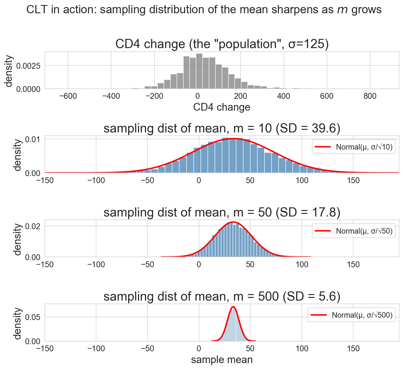
draw samples of size m from CD4 data

four panels: population, m=10, m=50, m=500

Anchor the symbol set before the demo: one card that groups n_T, n_C (actual trial sizes), m (the knob we’re turning in this demo), and B (outer-loop count — how many resamples, not sample size). CLT scales with m, not with B. Four-panel demo. Top-left: the population distribution \mathcal{X} of individual CD4 changes. Already fairly bell-shaped, because a cell count is itself an aggregate of many cell-level sources of variation. Top-right through bottom-right: the sampling distribution of the sample mean at m = 10, 50, 500. Three things happen as m grows: (1) the distribution centers more tightly on the population mean, (2) the spread shrinks like 1/m^{1/2} (quadruple m, halve the SD), (3) the shape converges to the red normal overlay. This is the CLT made visible.

standard error — the width of the sampling distribution

CLT \Rightarrow \text{SE}(\bar X) = \dfrac{\sigma}{m^{1/2}}

in practice: we don’t know \sigma — substitute the sample SD s

\widehat{\text{SE}}(\bar X) = \dfrac{s}{m^{1/2}}

m	SE from formula	SE from simulation
10	39.6	39.6
50	17.7	17.8
500	5.6	5.6

formula and simulation agree — CLT isn’t just a theorem, it’s a tool

Check the CLT formula against simulation. Compute SE = σ/√m for each of the three sample sizes, compare to the empirical SD of the 10,000 means at that sample size. They agree to within a percent. The formula is not just descriptive — it’s predictive. Given the population SD and a sample size, we can compute the SE directly, no resampling needed. That’s the setup for the normal approximation coming next.

the normal approximation

if the bootstrap distribution is normal, we don’t need 10,000 resamples

\hat{\theta} \pm 1.96 \cdot \widehat{\text{SE}}

for one mean: \widehat{\text{SE}} = s / n^{1/2}

for a difference: variances add (groups are independent, thanks to randomization)

\widehat{\text{SE}} = \left(\frac{s_T^2}{n_T} + \frac{s_C^2}{n_C}\right)^{1/2}

Here’s the payoff, staged one fragment at a time. Stop at each reveal and ask students to predict the next step before uncovering it. Fragment 1 — “if the bootstrap distribution is normal, we don’t need 10,000 resamples.” Ask: if the distribution is normal, what piece of it do we actually need? Fragment 2 — point estimate plus/minus 1.96 SE. One line of code instead of 10,000 resamples. Fragment 3 — one-mean SE, s/n^{1/2}, plug-in version of the CLT result we just established. Ask: we have two group means here; how do we combine their SEs? Fragment 4 — variances add because the two groups are independent (randomization buys us that independence). Fragment 5 — SE of the difference, a square-root of summed variances each divided by their group size. Walk the algebra slowly so the “variances add” claim lands before the formula arrives.

bootstrap vs formula — head to head

approach	\widehat{\text{SE}}	95% CI
bootstrap, 10,000 resamples	5.6	[39.6, 61.3]
normal formula	5.6	[39.6, 61.2]

both columns estimate the true SE — write \widehat{\text{SE}}

they agree — so why do we teach both?

Side-by-side. Bootstrap and formula give almost identical CIs — they differ by a tenth of a CD4 cell. The small gap is Monte Carlo error from the finite 10,000 resamples. So the question students should be asking: why bother with 10,000 resamples if one formula gets the same answer? The answer comes in two parts: (1) the formula is better when it works — faster, composable, lets you do power calculations; (2) the formula stops working for a big class of statistics, and the bootstrap doesn’t.

when to reach for the normal approximation

advantages:

• analytical planning — “how many patients to detect a 50-cell effect?” needs the formula, not resampling
• composable — combine SEs across studies, e.g. meta-analysis
• speed + less code — one line vs 10,000 resamples

the real reason to teach the formula: the questions it answers that the bootstrap can’t

Four advantages. The first is the killer one: before the trial ran, NIH had to answer “how many patients must we enroll to detect a 50-cell effect with 80% power?” That question requires inverting the SE formula — you don’t have data yet, so there’s nothing to bootstrap. Power calculations are a major application in trial design (Ch 10). The second is meta-analysis: given SEs from multiple studies, you can combine them directly if each was computed from a formula. Speed and simplicity are real but smaller gains.

analytical planning — how big a trial?

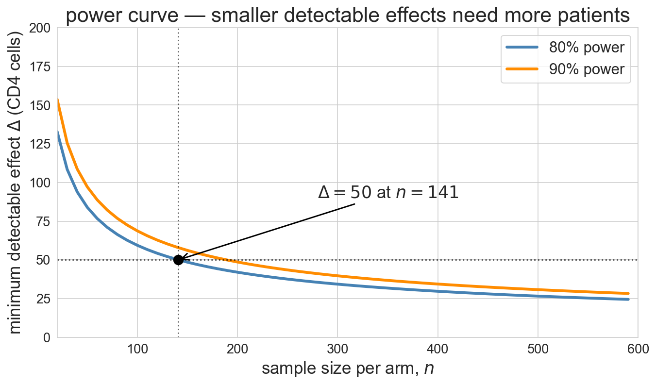
before ACTG 175 enrolled a patient, NIH had to answer: how many patients?

• target detectable effect: \Delta = 50 CD4 cells
• illustrative SD guess from pilot data: \sigma \approx 150 per arm
• 80% power
• significance \alpha = 0.05

z_{\alpha/2} = 1.96 (two-sided 5% critical value), z_\beta = 0.84 (80th percentile of N(0,1))

n \;=\; \frac{2\sigma^2 \,(z_{\alpha/2} + z_\beta)^2}{\Delta^2} \;=\; \frac{2 \cdot 150^2 \cdot (1.96 + 0.84)^2}{50^2} \;\approx\; 141 \text{ per arm}

formula assumes equal group sizes — trial design choice

bootstrap can’t do this — no data yet to resample

Concrete case study of the analytical-planning advantage. The power curve shows the tradeoff: smaller detectable effects need more patients, and the rate is 1/\sqrt{n}. ACTG 175’s 50-cell target at 80% power requires n ≈ 141 per arm (marked with dot); halving the target to 25 cells would require ~560 per arm. Before NIH could fund ACTG 175, they had to answer: how many patients? Targeted 50 CD4 cells as the minimum clinically meaningful effect. Guessed σ ≈ 150 per arm from pilot data and prior trials. Wanted 80% power — the probability of correctly declaring an effect if the true effect is 50 cells — at α = 0.05. Plug into the power formula and it pops out around 141 per arm, call it 280 total. ACTG 175 actually enrolled 2,139 patients, roughly ten times the floor, because they wanted to detect smaller effects and support subgroup analyses. But the main point is: this calculation requires the formula. The bootstrap can’t do it — there’s no data yet to resample. Chapter 10 formalizes power once we have hypothesis testing.

for each statistic, predict: does the formula work, marginal, or fail?

• works — formula CI matches bootstrap
• marginal — formula CI slightly off in shape or coverage
• fails — formula CI badly wrong, or no formula exists

then classify:

• mean of 500 Airbnb prices
• median of 500 Airbnb prices
• max of 500 Airbnb prices
• mean of 20 Airbnb prices

DISCUSSION: Per-statistic prediction (4 min — 2 min commit to works/marginal/fails for each of the four, then share with a neighbor). Prompt: For each of the four statistics, decide: formula works, marginal, or fails? Process goal: force all four evaluations — not just spotting the “weird” one. Students must reason about CLT applicability, heavy tails, and extreme quantiles separately. Expected answers: - mean of 500 prices: works — the CLT has kicked in even for skewed Airbnb data; normal CI and bootstrap CI agree. - median of 500 prices: fails — no simple closed-form SE; the median’s asymptotic SE involves the population density at the median, which you’d need another bootstrap to estimate. Reach for the bootstrap directly. - max of 500 prices: fails — extreme quantiles carry little information in the tails, and no resampling method conjures information the data doesn’t have. Both formula and bootstrap struggle. - mean of 20 prices: marginal — CLT is slow to kick in for heavy-tailed prices at small n; the bootstrap distribution is visibly skewed. Formula CI will be symmetric when truth isn’t, so it’s in the wrong direction by a few %. Bootstrap is better but not magic. If stuck: “Which statistics have a nice SE formula? Which live on the boundary of the data?” Key insight: the bootstrap extends our reach from ‘means of large samples’ to ‘any statistic’ — but no resampling method conjures information the data doesn’t have, so extreme quantiles are beyond both tools. Next slides: failure mode 1 (median) and failure mode 2 (heavy tails) verify the ranking with demos.

failure mode 1 — the median

CLT applies to means, not medians

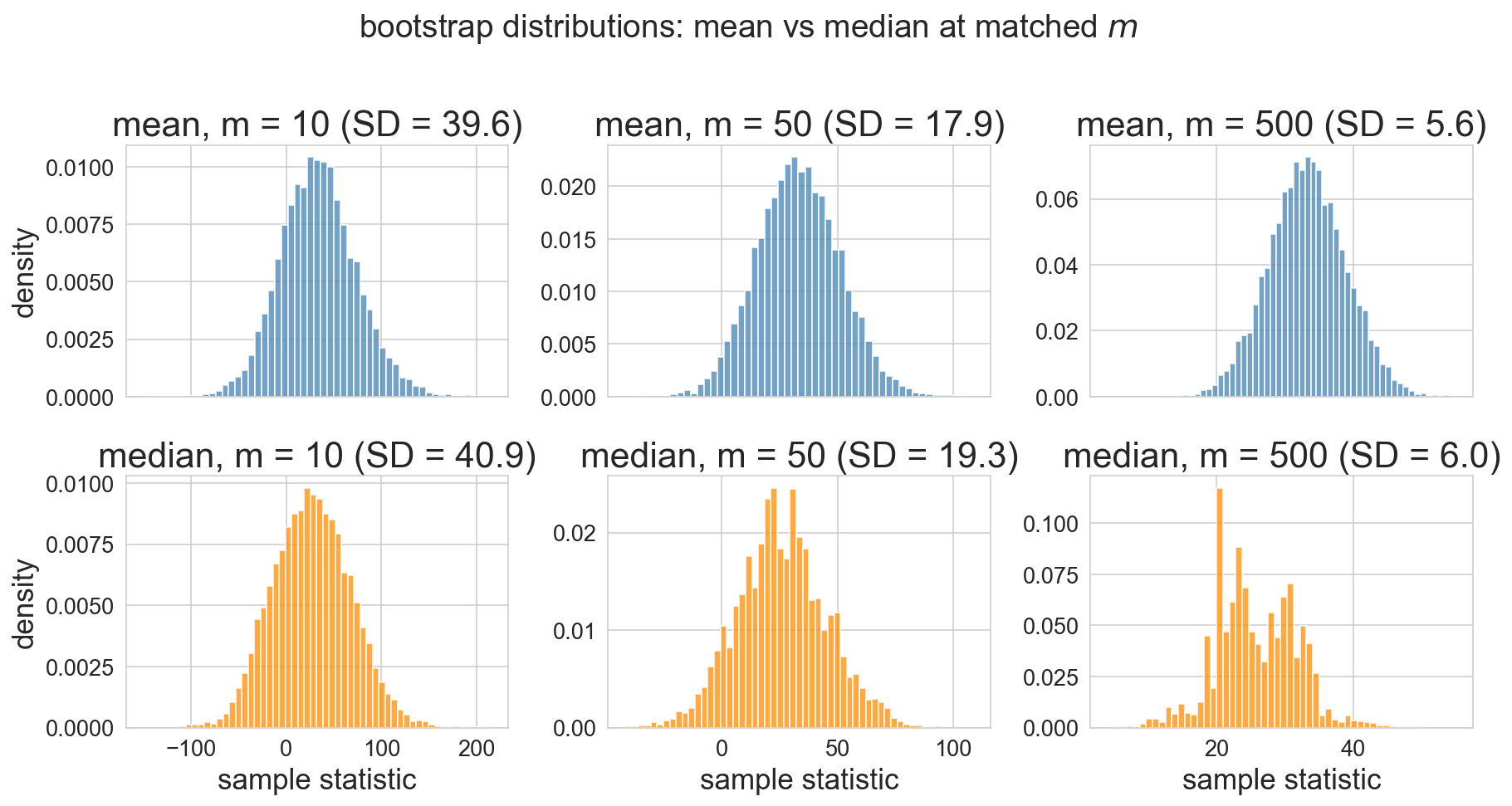
median’s bootstrap distribution is lumpier, wider, no simple closed-form SE

Demo 1 of when the normal approximation fails. Bootstrap the mean and bootstrap the median at matched sample sizes. At m=10 the median’s bootstrap distribution is visibly discrete — the sample median can only take values that actually appear in the resample, so its distribution lives on a grid of the order statistics. The CLT does not apply to order statistics in the same clean way it applies to sums. There’s an asymptotic formula for the median’s SE, but it involves the unknown population density at the median — you’d essentially need another bootstrap to estimate it. For the median, the bootstrap is the only practical tool.

failure mode 2 — heavy tails at small m

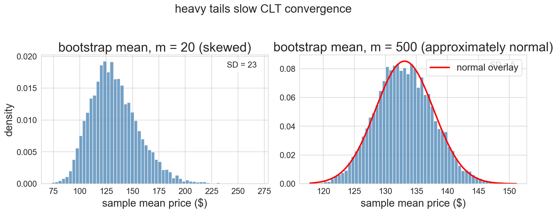
m=20 with right-skewed prices: bootstrap itself is skewed — normal CI would lie

m=500: CLT has kicked in

Demo 2. Bootstrap the mean of Airbnb prices — a famously heavy-tailed distribution (mean $133, median $100, max $999). At m=20 the bootstrap distribution of the mean is visibly right-skewed because even averaging 20 heavy-tailed draws isn’t enough for the CLT to kick in. A normal-approximation CI here would be symmetric around the point estimate, which is wrong — the true uncertainty is asymmetric. At m=500, the CLT has caught up and a normal fits fine. Heavy tails slow convergence; the “large enough n” in the CLT statement is bigger than you’d think.

caveat — bootstrap isn’t magic either

• tiny n: observed sample is a bad picture of the population — bootstrap inherits the flaw
• extreme quantiles — min, max, 99th percentile — data carries little info in the tails
• rule of thumb:
  • m \geq 30 for mild skew
  • m \geq hundreds for heavy tails

when the bootstrap distribution looks wrong, the CI is a warning — not an answer

Walk back the “bootstrap always works” impression. It’s the right tool when you can’t derive a formula, but it still needs enough data for the observed sample to be representative. With n=5, there’s nothing to resample that the formula doesn’t also fail on. And for extremes — 99th percentile, max — even a large sample has few observations in the tails, and resampling amplifies that sparsity rather than fixing it. Rule of thumb: 30 for gently skewed data, hundreds for heavy tails. More importantly: look at the bootstrap distribution. If it’s visibly lumpy, skewed, or chopped-off, the CI is giving you a diagnostic, not a final answer.

you’re the PM — should you ship the new checkout?

the same tools scale beyond clinical trials — here’s one you’ll face in industry

A/B test: half your users see the old checkout, half see the new

the results are in:

• lift: +2.1% sign-ups
• 95% bootstrap CI: [+0.3%, +3.9%]
• new flow: more complex, adds 2 external dependencies

ship it? defend:

• what the CI shows — and what it doesn’t catch
• cost and maintainability: is +2% worth +2 dependencies?
• is more data worth waiting for?

DISCUSSION: Capstone decision (4 min — commit to ship/wait/don’t ship, defend in pairs using all three considerations). Prompt: Should you ship the new checkout flow? Process goal: force synthesis — the CI is necessary but not sufficient. Real decisions require weighing statistical evidence against cost, risk, and operational reality. This is the first slide in the course using “A/B test” terminology; the inline gloss (“half your users see the old, half see the new”) is the operational definition. If students haven’t heard the term, that’s fine — the setup is self-contained.

The straightforward statistical read: 95% CI [+0.3%, +3.9%] excludes zero, so the lift is “real” by bootstrap logic. Ship? Not so fast.

What the CI doesn’t catch: - Systematic shifts: seasonality, novelty effects (users click the new thing because it’s new, not because it’s better), holiday spikes. The CI covers user-to-user noise under the same conditions, not conditions changing. - Subgroup effects: aggregate +2% might mean +4% for new users and -0.5% for returning users — shipping hurts the returning cohort. - Implementation risk: the A/B test ran on current infrastructure; full deployment may interact with other systems differently.

Cost and maintainability: - +2% sign-ups is material only if your base is material. 2% of 1M monthly users is different from 2% of 1,000. - 2 external dependencies = ongoing security patching, version-upgrade burden, slower build and CI pipelines. That cost compounds over years. - General principle: the simpler option wins unless the complex one offers enough gain to pay its maintenance tax.

Would more data help? Yes — another week would narrow the CI. But waiting costs too: opportunity cost of the lift not captured, team momentum, context switching back later. The disciplined answer: set a threshold in advance (“ship if CI lower bound > 1%”) and commit rather than negotiate with yourself.

Three defensible answers: - “Ship but monitor”: CI above zero, cost manageable, define kill-switch metrics (if sign-ups drop by X% post-launch, revert). - “Wait 2 more weeks”: CI lower bound is 0.3%, uncomfortably close to zero; more data de-risks and the lift’s there to be had. - “Don’t ship”: the ongoing cost of 2 dependencies exceeds the expected +2% lift, especially if the +2% is inflated by novelty.

All three are defensible. What matters is the reasoning — not pattern-matching to a CI-excludes-zero heuristic. Ties back to the “what a CI does and doesn’t cover” slide in Block 2 and forward to Chapter 16 (backtesting), where models trained under conditions X fail under conditions Y.

If stuck: “The CI excludes zero — so ship? Good, now push harder: what kinds of failure would the CI miss?”

one dataset, one statistic, quantified uncertainty

summary

• bootstrap = resample with replacement to approximate the sampling distribution
• CLT = why bootstrap distributions of means look normal
• normal approximation = \hat{\theta} \pm 1.96 \cdot \text{SE} when CLT applies — fast, composable, powers trial design
• reach for bootstrap when the statistic isn’t a mean, tails are heavy, or n is small
• neither tool is magic: extreme tails, tiny samples — no method conjures missing information

Five takeaways that map to the four agenda beats. The bootstrap is a general recipe for any statistic. The CLT is why the special case of means has a clean formula. The normal approximation is the fast path when the CLT applies. The bootstrap is the fallback when it doesn’t. And neither is a cure-all — extreme quantiles and tiny samples break both tools. Where students will meet this outside stats class: A/B testing (every feature ship decision at a tech company), poll aggregation (FiveThirtyEight-style election forecasts), financial risk (value-at-risk from bootstrapped return distributions). Same recipe everywhere: one dataset, one statistic, a CI.

next time

• Ch 9: permutation tests — bootstrap quantified the estimate, permutation asks: could the effect be zero?
• Ch 10: the hypothesis-testing framework formalizes both
• Ch 12: bootstrap for regression coefficients

Forward pointer. The bootstrap answered “how precise is the treatment effect?” and gave us a CI. Chapter 9 answers a related but distinct question: “could the effect plausibly be zero?” That’s what permutation tests are for — shuffle the treatment labels, rebuild the sampling distribution under the null, and see how extreme the observed effect is. Chapter 10 formalizes hypothesis testing in general. Chapter 12 returns to bootstrap and applies it to regression — same recipe, bigger statistic.

one-minute feedback

1. what was the most useful thing you learned today?
2. what was the most confusing?

give feedback

Closing ritual. Keep the slide up until the room clears.