Lecture 7: Classification — Logistic Regression and Metrics

MSE 125 — Applied Statistics

Madeleine Udell

Monday, April 20, 2026

logistics

• quiz 3: Wed April 22 — Lec 6-7 (validation + classification)
• HW 2: due Fri April 24 — regression, validation, classification
• project proposal: due Fri May 1

START RECORDING.

Thirty-second logistics check. Quiz Wednesday covers last lecture (validation, bias-variance) and today (classification metrics). HW 2 Friday leans on today’s material for the Framingham portion. Project proposal due end of the following week.

a model is 85% accurate

does it catch the patients who need it?

Open with the hook. A hospital wants to flag patients likely to be readmitted within 30 days so it can intervene. It trains a fancy classifier. It reports 85% accuracy. Deploy it, right? Pause. Then the kicker: the model predicts “no readmission” for every patient. That 85% accuracy is just the base rate. Today’s lecture is why accuracy lies when one class dominates — and what to use instead.

the readmissions setup

the problem

• hospital wants to flag 30-day readmissions
• missed readmission costs up to $25,000 in care
• CMS penalizes hospitals with excess readmission rates — up to 3% of total reimbursements

the data

• 15% of patients get readmitted
• 85% don’t
• predict “no readmission” for everyone →
• 85% accuracy

the dumbest possible model beats random, passes QA, and saves zero lives

Why we care: readmissions are expensive both clinically and in penalty dollars. But the base rate is 15% positive, which makes the null-model baseline look like a good model on any accuracy-based evaluation. This is our motivating setup. We’ll fit a real classifier on the same kind of data (Framingham CHD — same 15% base rate), discover the same trap, and build a toolkit of metrics that actually tell us whether the model is doing anything useful.

today

• the mechanics: logistic regression, gradient descent
• the evaluation trap: why accuracy lies
• threshold choice: no free lunch
• what accuracy hides: base rates, subgroups, calibration

Four blocks. First: the mechanics — how do we actually fit a classifier? Second: the evaluation trap we opened with. Third: threshold choice as a cost-benefit decision, not a statistical one. Fourth: three ways a model can “work on paper” while being useless in practice — base rate neglect, subgroup failure, miscalibration.

first we need a classifier

the outcome is binary

Framingham Heart Study: 4,240 patients, 10-year followup

• started in 1948 in Framingham, Massachusetts
• first study to identify cholesterol, blood pressure, and smoking as heart disease risk factors
• still running — now on its third generation of participants

outcome: TenYearCHD \(\in \{0, 1\}\) — did the patient develop coronary heart disease within 10 years?

• CHD = 1 — positive class
• no CHD = 0 — negative class

“positive” = the outcome we’re trying to detect, not the desirable one

Our running example for the lecture. Framingham is the landmark cardiovascular study from 1948 that identified cholesterol and blood pressure as risk factors. The outcome we’ll try to predict is whether a patient develops coronary heart disease within ten years. That outcome is binary — 1 if CHD, 0 if not. And about 15% of patients are CHD-positive, same as our readmissions hook. Quick vocabulary stake: the class we try to detect is the “positive” class. The terminology originated in signal detection theory (radar, sonar) and was adopted by medical testing — a positive result is one that detects the condition — it’s bad news for the patient, not good news. That distinction will matter when we talk about sensitivity and specificity.

can we just run linear regression?

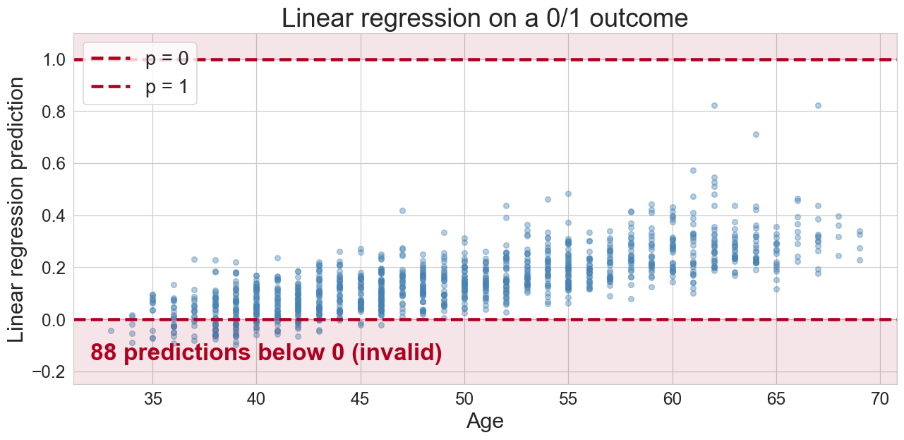
predictions below 0 and above 1 — not valid probabilities

The obvious first attempt: fit OLS to the 0/1 labels. It runs. But the predictions are nonsense — many are negative, some exceed 1. Nothing constrains OLS to produce numbers in [0, 1]. We need a model that lives on the probability scale.

the trick: squeeze the line through a sigmoid

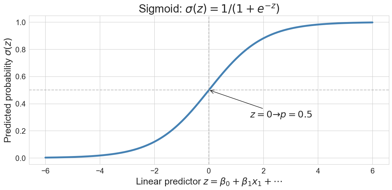
\[p = \sigma(z) = \frac{1}{1 + e^{-z}}, \quad z = \beta_0 + \beta_1 x_1 + \cdots + \beta_d x_d\]

Rather than constrain OLS, transform what we want to model. The linear predictor z = β₀ + β₁x₁ + ⋯ can be any real number. Push it through the sigmoid σ(z) = 1/(1+e⁻ᶻ) and the output is forced into (0, 1). The sigmoid is symmetric around zero: z = 0 maps to p = 0.5, big positive z maps toward 1, big negative z maps toward 0. Logistic regression is just linear regression on the log-odds of the outcome, then squashed through σ.

sports bettor’s intuition

sportsbook: “the Celtics are 4-to-1 underdogs tonight”

Q: what probability of winning does that imply?

odds \(= \dfrac{P(\text{win})}{P(\text{lose})}\)

4-to-1 against → lose 4 games per 1 win → \(P(\text{win}) = \tfrac{1}{1+4} = 0.20\)

probability in \([0, 1]\) \(\leftrightarrow\) odds in \([0, \infty)\) — same info, different scale

Probe for prior knowledge. Most students have seen “3-to-1 odds” in sports, poker, or general English. Odds = P(win) / P(lose). 4-to-1 against means for every 1 win there are 4 losses, so P(win) = 1/5 = 0.20. The probability-odds correspondence is one-to-one — anything you can say about probabilities you can say about odds. The useful move is next: take the log and the range opens up further.

from probabilities to log-odds

probability \(p\)	odds \(p/(1-p)\)	log-odds
0.01	0.01	\(-4.6\)
0.20	0.25	\(-1.4\)
0.50	1.00	\(\phantom{-}0.0\)
0.80	4.00	\(+1.4\)
0.99	99.0	\(+4.6\)

log-odds range from \(-\infty\) to \(+\infty\) — perfect for a linear model

\[\log\frac{p}{1-p} = \beta_0 + \beta_1 x_1 + \cdots\]

Same math, different way to see it. Odds = p / (1-p), familiar from sports betting. Odds range from 0 to infinity. Take the log and the range opens up to the full real line. That’s what we model with a linear function of x. The log-odds are called the logit, and logistic regression is the claim that the logit is linear in the features.

check your intuition

Pr(Win) = 0.6 → odds = \(\frac{0.6}{0.4} = 1.5\)

I double your odds → new odds = 3.0

Q: new Pr(Win) = ?

\[\text{Pr(Win)} = \frac{3.0}{1 + 3.0} = 0.75\]

doubling odds \(\neq\) doubling probability — the scales are nonlinear

INLINE Q/A: Think-pair-share (3 min) Prompt: Pr(Win) = 0.6. I double the odds. What’s the new probability? Process goal: compute on a nonlinear scale Common wrong answer: “1.20” (doubled 0.6) — breaks immediately since probabilities can’t exceed 1. Subtler wrong answer: “0.80” from vague doubling logic. The correct answer (0.75) requires converting to odds, doubling, converting back. If stuck: “Convert to odds first — what are the odds when Pr(Win) = 0.6?” Key insight: This is why logistic regression coefficients are hard to interpret on the probability scale: a one-unit increase in a feature multiplies the odds by \(e^\beta\), but the effect on probability depends on where you start.

logistic regression on age alone

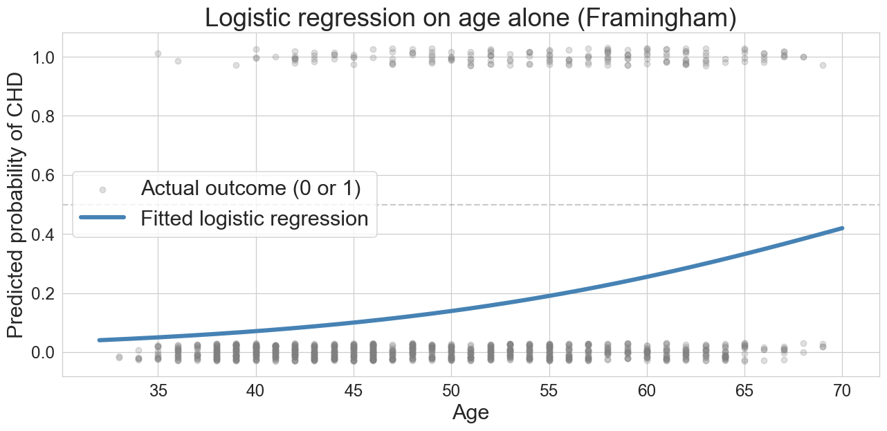
predicted risk climbs with age — we see the lower portion of the S-curve because the base rate is low

Fit logistic regression with just age as the feature so we can plot the whole decision curve. The curve rises from under 5% for the youngest patients to over 30% for the oldest. We’re looking at the lower tail of the S — the full sigmoid would sweep through 0.5 and level off at 1, but the base rate of CHD is low enough that age alone doesn’t get anyone to 50% predicted risk. When we add more features, each patient’s predicted probability depends on nine risk factors, not just age — and no one feature tells the whole story.

where does the loss come from?

MLE (maximum likelihood estimation): pick \(\beta\) to makes observed labels most probable

for one observation with label \(y \in \{0, 1\}\) and predicted probability \(p\):

\[P(y \mid x) = p^{\,y} \, (1-p)^{1-y}\]

likelihood of \(n\) observations. independent, so multiply:

\[L(\beta) = \prod_{i=1}^n p_i^{\,y_i} \, (1-p_i)^{1-y_i}\]

take \(-\log\): products → sums, maximize → minimize

\[-\log L(\beta) = -\sum_{i=1}^n \big[ y_i \log p_i + (1-y_i) \log(1-p_i) \big]\]

Every loss function comes from somewhere — usually a modeling assumption. For logistic regression, the loss drops out of maximum likelihood. Treat each label as a Bernoulli draw with parameter p = σ(xβ). The per-observation probability is p^y (1-p)^(1-y): evaluates to p if y=1, to (1-p) if y=0. Multiply across independent observations to get the likelihood. Take the log to turn products into sums, then negate — maximizing likelihood becomes minimizing negative log-likelihood, which is the log loss. So the loss isn’t pulled out of a hat — it’s the direct consequence of assuming Bernoulli labels.

the logistic loss

\[\ell(\beta) = -\big[ y \log(p) + (1-y) \log(1-p) \big]\]

also called cross-entropy or negative log-likelihood

penalizes confident wrong predictions especially hard

• \(y = 1\), \(p \to 0\): \(-\log(p) \to \infty\)
• \(y = 0\), \(p \to 1\): \(-\log(1-p) \to \infty\)

Q: if \(y = 1\) and \(p = 0.9\), loss = \(-\log(0.9)\) ≈ ? what about \(p = 0.1\)?

• \(-\log(0.9) = 0.11\) (confident, correct → small)
• \(-\log(0.1) = 2.3\) (confident, wrong → large)

no closed-form minimum. we’ll need an iterative solver.

Quick computation to anchor the formula before the visual comparison. The single-observation form of the loss. If the label is 1 and we predicted p, the loss is -log(p); if the label is 0, it’s -log(1-p). Either way, the loss is small when we’re right with high confidence and large when we’re wrong with high confidence. “Confident wrong” is punished severely — that’s why logistic regression picks coefficients that aren’t overconfident on hard cases. Unlike linear regression, there’s no closed-form minimum — the sigmoid makes the gradient nonlinear in β. That motivates gradient descent on the next slide.

squared error vs. logistic loss

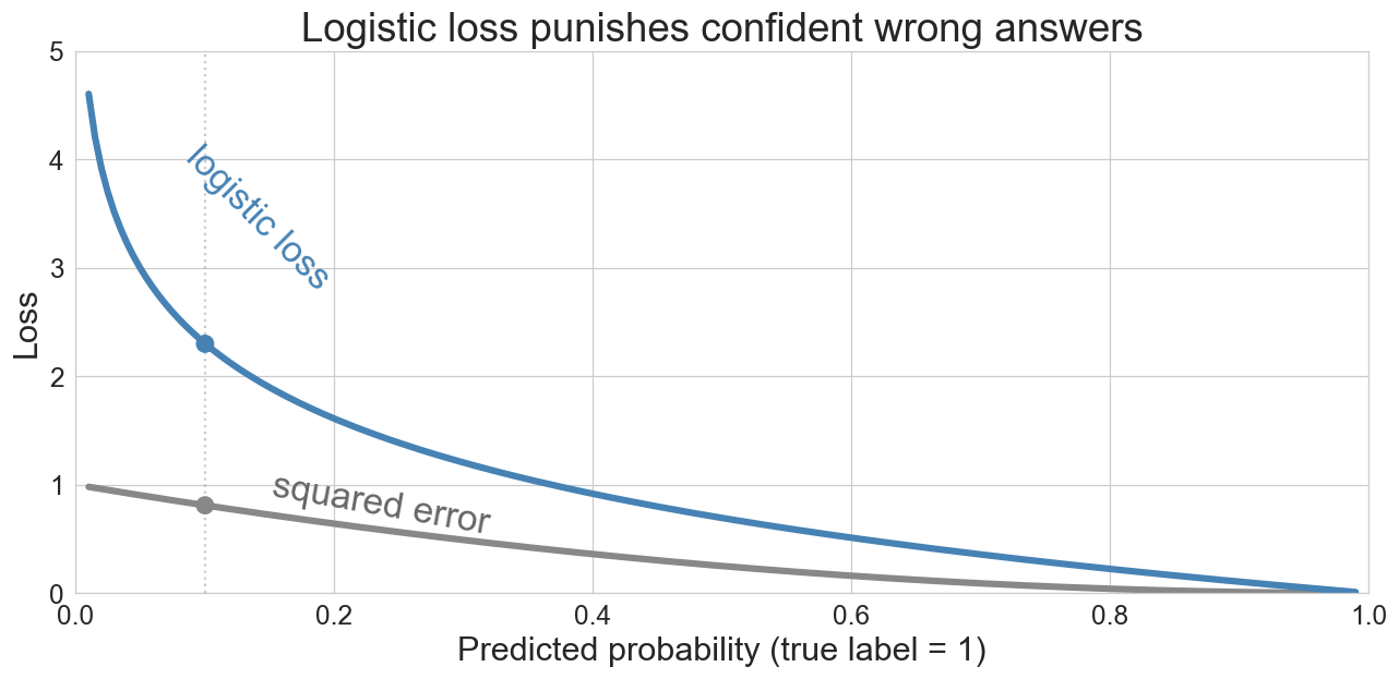
a 10% prediction for a true 1? squared error 0.81, logistic loss 2.3

the loss function determines what the model finds

The comparison visually. When the prediction is near 1 (correct, confident), both losses are small. As the prediction drops toward 0 for a true 1 — a confident wrong answer — squared error stays below 1, but logistic loss explodes. That asymmetry is what forces logistic regression to avoid overconfidence on hard cases. The one-liner: the loss function determines what the model finds. Choose squared error and the model minimizes average distance; choose logistic loss and the model minimizes confident-wrong predictions. The loss is a design choice, not a given.

gradient descent: hiking downhill

\[\beta \leftarrow \beta - \eta \cdot \nabla L(\beta)\]

• \(\nabla L(\beta)\) = gradient (uphill direction); step the opposite way
• \(\eta\) = learning rate (step size)

logistic loss is convex — one valley, no false minima

Picture the loss as a landscape over the β coefficients. Gradient descent is literal hiking. At each step, compute the gradient — the vector of partial derivatives, which points uphill — and step the opposite direction. η is the step size. Too small and it’s slow; too big and you overshoot. The magic property of logistic regression is that the landscape is convex: a single bowl with no false valleys. Gradient descent finds the global minimum regardless of starting point. Callback: in Chapter 5, linear regression had the normal equations — a closed-form solution. The sigmoid makes the loss nonlinear in β, so there’s no formula. We iterate instead. Edge case worth mentioning if a student asks: if the data is perfectly separable (a line can perfectly separate the two classes), the sigmoid can always be pushed closer to 0 or 1, so coefficients grow without bound and no finite minimum exists. The loss is still convex — it’s the minimum that runs off to infinity.

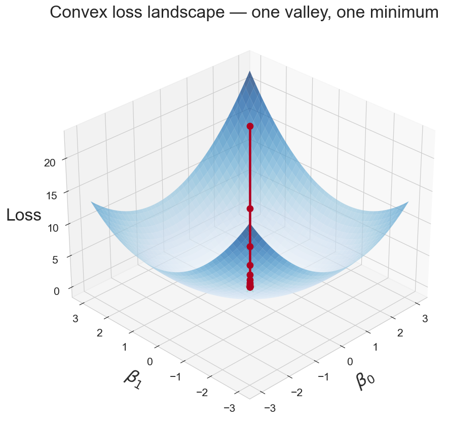
watch it converge

Q: will the loss curve drop smoothly, oscillate, or bounce around?

commit to a prediction — then we run 50 iterations

INLINE Q/A: Predict-then-reveal (1 min) Prompt: Will the loss curve drop smoothly, oscillate, or bounce around? Process goal: predict convergence behavior from convexity Common wrong answer: “oscillate” — reasonable, since gradient descent can oscillate with too-large a step size. But with η = 0.5 on a convex problem, we’ll see smooth descent. If stuck: “We said the loss is convex — one valley. Does that help?” Key insight: The commitment matters more than the answer — students who predicted the wrong shape will remember the reveal.

watch it converge

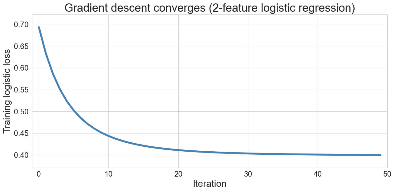
50 iterations on age + BMI (body mass index) logistic regression. loss drops fast, then settles.

Reveal. The loss drops sharply in the first handful of iterations, then settles. Because the problem is convex, “settles” means we’ve found the minimum. sklearn’s LogisticRegression uses a fancier variant (L-BFGS or similar), but the intuition is the same: start somewhere, step downhill, stop when the gradient is small.

accuracy lies under class imbalance

fit it, test it

# setup: Framingham data, 9 features, standardized, 70/30 split
model = LogisticRegression(penalty=None, max_iter=1000).fit(X_train_scaled, y_train)
test_acc = model.score(X_test_scaled, y_test)
print(f"Test accuracy: {test_acc:.2f}")

Test accuracy: 0.855

85.5% accurate (at default threshold 0.5) — sounds great, right?

Fit our 9-feature logistic regression on the Framingham training set — the full feature set, with standardized features. Compute accuracy on the held-out test set. 85.5%. A B+ on a typical grading curve. Hold this number in mind. Now: what’s the accuracy of the dumbest possible model?

but wait

the “always predict no CHD” baseline:

Q: what accuracy does it get?

baseline accuracy  = 0.848
our model accuracy = 0.855
improvement        = 0.007

our fancy classifier barely beats the null

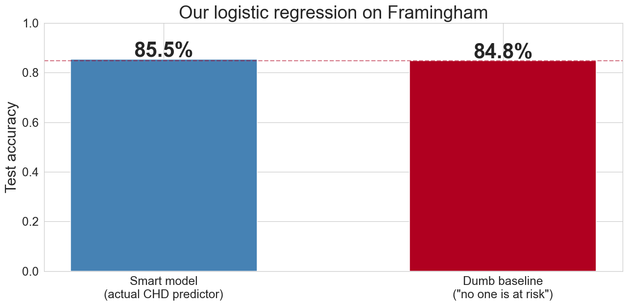
accuracy measures how often you’re right overall — when one class dominates, that’s easy and uninformative

Predict “no CHD” for every single patient — no features, no fitting, nothing. Its accuracy is 1 - base rate = 85% because 85% of patients actually don’t develop CHD. Our model’s 85.5% is only slightly better. The 85.5% accuracy number was almost entirely driven by class imbalance, not by the model learning anything useful. This is the accuracy trap — and it shows up whenever one class dominates. Accuracy is a population-averaged metric, weighted by how often each class appears. In an imbalanced problem (medical screening, fraud, equipment failure, spam), the common class dominates the average. Metrics that weight the two classes differently — or that look at each class separately — tell a more honest story. We need different metrics.

the confusion matrix

1,096 test patients · 15% CHD base rate · threshold 0.5

	predicted no CHD	predicted CHD
actually no CHD	TN (true negative) = ?	FP (false positive) = ?
actually CHD	FN (false negative) = ?	TP (true positive) = ?

predict: of 167 actual CHD cases, how many does the model catch?

• fewer than 20
• 20–50
• 50–100
• more than 100

INLINE Q/A: Poll (1 min) Prompt: Of 167 actual CHD cases, how many does the model catch? Process goal: predict a magnitude Common wrong answer: “50–100” or “more than 100” — students anchor on the 85% accuracy and assume the model catches most cases. The real answer (17) is shocking. Most students will pick too high, which sets up the precision/recall reveal perfectly. If stuck: “The model is very conservative — it predicts ‘no CHD’ for almost everyone. What does that mean for the bottom row?” Key insight: The TN cell dominates. The model gets 85% accuracy by correctly predicting the easy cases and missing almost all the hard ones.

the confusion matrix

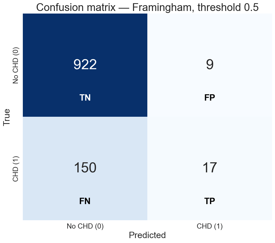
of 167 actual CHD cases, we caught 17

Reveal. True negatives dominate (922) — exactly as predicted. But the bottom row is the story: 17 caught, 150 missed. The model is correctly saying “not CHD” to most people and missing the ones that matter. Accuracy hid this because the 922 true negatives drown out everything else.

precision vs. recall

precision \[\frac{\text{TP}}{\text{TP} + \text{FP}}\]

“I flagged this patient — should I trust the flag?”

recall (sensitivity) \[\frac{\text{TP}}{\text{TP} + \text{FN}}\]

“of all the sick people, how many did we find?”

F1 score = harmonic mean of precision and recall — one number, but hides the cost asymmetry

two metrics → two different stories

Precision is the precision of your positive predictions — when you say yes, how often are you right? Recall is the completeness of your positive detection — of all the true positives out there, how many did you catch? They move in opposite directions when you change the threshold. Require higher confidence before flagging → precision up, recall down. Lower the bar → more flags, precision drops, recall climbs.

our model’s precision and recall

Precision: 0.65
  → Of patients flagged as CHD, 65% actually had it

Recall:    0.10
  → Of actual CHD patients (167 in test set), we caught 17

accuracy hid a disaster — the model catches almost nobody

Precision is decent — when the model does flag someone, about two-thirds of the time it’s right. But recall is abysmal. Of all 167 actual CHD patients in the test set, we caught 17. For a screening tool this is a complete failure. The 85% accuracy masked that the model is barely functioning on the task we actually care about.

which type of error would you rather the model make?

• CHD screening:
  • FP → $500 follow-up
  • FN → $50K emergency care
• spam filter:
  • FP → real email lost → missed meeting
  • FN → spam in inbox → mild annoyance

for each: flag more, or flag fewer?

DISCUSSION: Think-pair-share (3 min — 30 sec think, 1 min neighbor). Prompt: Which type of error would you rather the model make — for CHD screening and for spam? Process goal: cost-benefit reasoning about asymmetric errors Common wrong answer: students who focus on the medical case may say “FP is also bad because of patient anxiety” — valid, but the dollar asymmetry (500x) makes FN clearly worse. The interesting split comes from students who reason differently about spam vs. medicine. If stuck: “Start with medicine. A missed heart attack costs $50K. A follow-up test costs $500. Which mistake is cheaper?” Key insight: The right threshold depends on the business problem, not the statistics. Threshold choice is a cost-benefit call. Callback: “positive” = condition detected, not condition desired. A false positive means we flagged someone who is actually healthy.

when is a flag worth it?

flag if the expected savings beat the expected cost

flag whenever P(disease | flagged) > break-even precision

\[p^* = \frac{1}{k+1}\]

where \(k = C_{FN}/C_{FP}\) is the cost ratio of a missed case to a false alarm

CHD: \(k = 100 \Rightarrow p^* \approx 1\%\) — push hard for recall

spam: \(k \ll 1 \Rightarrow p^* \approx 99\%\) — protect precision

Make threshold choice quantitative. For a single patient with predicted probability \(p\): flagging costs \((1-p)C_{FP}\) in expectation; not flagging costs \(p \cdot C_{FN}\). Flag when the first is smaller, which gives \(p > 1/(k+1)\) where \(k\) is the cost ratio. Call that threshold the “break-even precision” \(p^*\).

Why “precision” and not just “probability”? Because on the PR curve, precision IS the conditional probability \(P(\text{disease} \mid \text{flagged})\) — that’s the definition. So the rule reads off directly from the y-axis of the PR curve.

Two extreme calibrations: CHD has \(k=100\) ($50K vs $500), so \(p^* \approx 1\%\) — almost any flag is worth it. Spam has \(k\) much less than 1 (lost real email > extra spam), so \(p^* \approx 99\%\) — flag only when nearly certain.

If a sharp student asks “isn’t precision the average over flagged patients, not the marginal next flag?” — yes. The rule is slightly conservative because marginal precision sits below average precision. That’s fine — the cost ratio itself is an estimate, so a conservative margin is welcome.

precision-recall across thresholds

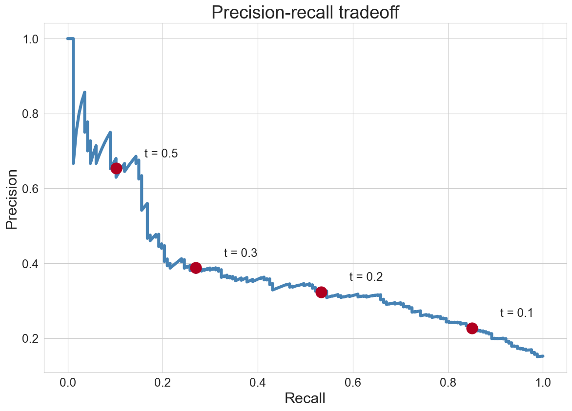
each annotated point is one threshold — as recall climbs, precision falls

precision is P(disease | flagged) — read the y-axis as trustworthiness of a flag

stop where precision still beats \(p^*\) — beyond that, the marginal flag loses money

Rather than pick a single threshold, sweep all of them. For each threshold, compute precision and recall and plot the point. Perfect model: a point at (1, 1). At t = 0.5 (top-left), precision is decent but recall is terrible. Slide down-and-right and you catch more real cases but each flag is less trustworthy.

Now apply the break-even rule from the previous slide. The y-axis literally is \(P(\text{disease} \mid \text{flagged})\) — that’s the definition of precision. So the rule “flag when \(P > p^*\)” translates directly to “stay above the horizontal line \(y = p^*\) on the PR curve.” Slide down the curve until precision approaches \(p^*\) and stop.

For our CHD model with \(k=100\), \(p^* \approx 1\%\) — every annotated point on this curve sits well above break-even, so the rule says push the threshold even lower than what’s plotted.

another view: ROC (receiver operating characteristic)

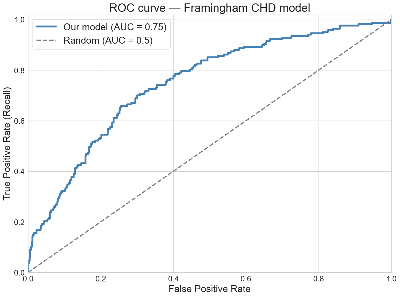
AUC (area under the curve) ≈ 0.75 — concordance: pick one CHD and one non-CHD patient; the model ranks the CHD patient higher 75% of the time (ties count as half)

Same threshold sweep, different axes: plot true positive rate (= recall) against false positive rate (= FP / all negatives). Perfect model: hugs the top-left corner. Random guessing: the diagonal. AUC = area under. Our 0.75 has a clean interpretation — concordance probability. Pick one CHD patient and one non-CHD patient; the model ranks the CHD patient higher 75% of the time. That’s threshold-free ranking quality. Let the 0.75 sit — the subgroup and calibration sections that follow will show why a decent aggregate AUC still hides trouble.

PR vs ROC — when to use which

PR curve

axes: precision · recall

depends on base rate

operational view — most honest when the positive class is rare

ROC curve

axes: TPR (true positive rate = recall) · FPR (false positive rate)

invariant to base rate

threshold-free summary (AUC) · compare models across datasets

same tradeoff, different invariances

Two cuts of the same threshold sweep. The PR curve speaks to the operational question — “when I flag a patient, am I right?” — which is exactly what matters in imbalanced screening. It depends on the base rate, so it’s not directly comparable across populations. The ROC curve and its AUC are invariant to how many negatives you have: shuffle in ten times more healthy patients from the same population and the ROC doesn’t change, while PR gets worse. (Caveat: if you move to a genuinely different population, the score distributions may shift and the ROC can change.) So for a fixed problem with a rare positive class — CHD, fraud, readmissions — the PR curve is usually the more honest view. For cross-dataset comparison or a ranking-quality summary, use ROC + AUC. In this class we’ll typically report both.

you’re reporting to the hospital board on your CHD model

do you show the PR curve or the ROC curve?

one-sentence justification

DISCUSSION: Think-pair-share (3 min — 30 sec commit to a curve, 1 min defend to a neighbor). Prompt: PR curve or ROC curve for the hospital board report? Process goal: apply the PR-vs-ROC distinction to a specific stakeholder Common wrong answer: “ROC because AUC is the standard metric.” Reasonable — but the board cares about operational performance on a rare condition (15% positive rate), and PR is the more honest view when the positive class is rare. ROC can look decent (AUC 0.75) while PR reveals the precision-recall tradeoff that drives staffing and follow-up costs. If stuck: “What question does each curve answer? Which question does the board care about?” Key insight: PR for operational decisions on rare conditions; ROC for comparing models across datasets. The audience determines the chart.

threshold effect on metrics

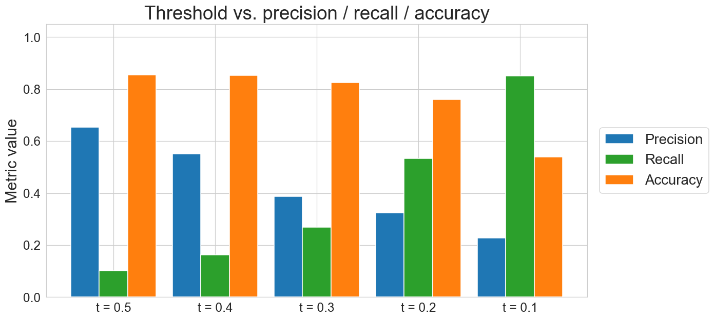
low threshold → catches more, but each flag is less reliable

Concrete numbers. At the default 0.5 threshold, accuracy is 86%, precision 65%, recall 10% — we flag only 26 of 1,096 test patients. Drop the threshold to 0.1 and we flag 624 patients (57% of the test set). Recall jumps to 85% — we catch almost all CHD cases — but precision drops to 23% (most flags are wrong) and accuracy falls to 54%, below baseline. What to pick? Depends on follow-up test cost, ICU bed availability, patient outcomes. No purely statistical answer.

aggregate metrics hide local failures

a vendor pitches a cancer screening test as 99% accurate:

• 99% sensitivity — catches 99% of cancer cases
• 99% specificity — correctly clears 99% of healthy patients

cancer prevalence: 0.5%

a patient tests positive — P(cancer | positive)?

A. 99% · B. 67% · C. 33% · D. 1%

DISCUSSION: Predict-then-reveal (3 min — commit by hands A/B/C/D, then work it out on 10,000 patients with a neighbor). Prompt: P(cancer | positive) given 99% sensitivity, 99% specificity, 0.5% prevalence? Process goal: Bayesian reasoning under base rate neglect Common wrong answer: A (99%) — most people anchor on the test accuracy and ignore the base rate. Even most doctors in published studies get this wrong (Casscells, Schoenberger & Graboys, 1978, NEJM). The correct answer is C (~33%). If stuck: “Start with 10,000 patients. How many actually have cancer at 0.5% prevalence? How many of those does the test catch? How many healthy patients does it falsely flag?” Key insight: False positives swamp true positives when the condition is rare. A “99% accurate” test yields only 33% PPV at 0.5% prevalence. Note: we’re being generous to the vendor by reading “99% accurate” as 99% sensitivity AND specificity. In practice, vendor claims often mean overall accuracy — achievable by predicting the majority class for everyone (the accuracy trap from earlier).

work it out on 10,000 patients

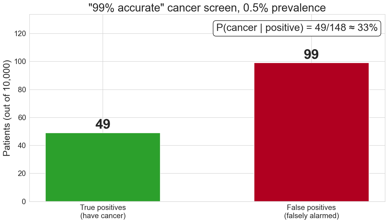
false positives swamp true positives when the condition is rare

Out of 10,000 patients: 50 actually have cancer (0.5% prevalence). Of those, the test catches 99%, so ~50 true positives. The other 9,950 are healthy. The test misclassifies 1% of them, so ~100 false positives. Total positive results: ~150. Of those 150, only ~50 are real — about 33%. The vendor’s “99% accuracy” number was true; the patient’s posterior probability was just 33%. That’s base rate neglect, and it’s why headline accuracy numbers on rare conditions are mostly meaningless.

aggregate AUC is 0.75 · recall: age is the model’s strongest signal

predict: which age group does the model fail on?

• under 40
• 40–54
• 55+

commit to a group — and say why

DISCUSSION: Predict-then-reveal (3 min — 30 sec commit to a group, 1 min defend to a neighbor). Prompt: Which age group does the model fail on, and why? Process goal: predict + explain mechanism Common wrong answer: “55+ because older patients are more complex / heterogeneous.” Reasonable — but wrong. The model does best on older patients because age is its dominant signal. Under-40 patients have AUC = 0.36 because the positive rate is tiny and age-as-signal carries no information. If stuck: “Think about where the model’s strongest signal — age — stops helping.” Key insight: Aggregate AUC hides subgroup failure. The model learned “older = riskier” and has nothing useful for young patients — exactly the group where early detection matters most.

subgroup AUC by age

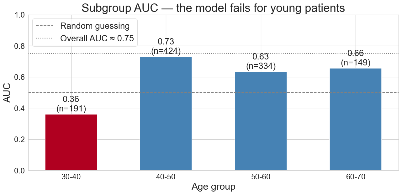
for patients under 40, AUC = 0.36 — below 0.5, but based on only ~6 CHD cases; the estimate is noisy

Compute AUC separately in each age group. For patients over 40, the model is decent — AUC above 0.6 across groups. For under-40 patients, AUC drops to 0.36 — below 0.5, worse than random guessing. Inverting the model’s ranking would actually do better in this subgroup. The positive class there is tiny — only ~6 CHD cases in 191 patients — so the estimate is noisy, but the message is unambiguous: the model has no useful signal for young patients. It learned “older people get heart disease” and nothing else. Side note worth making if time permits: the Framingham cohort is drawn from a historically homogeneous population (mostly white, one town in Massachusetts). The subgroup failure we see by age is just the beginning — a responsible deployment would also check performance by race, sex, and insurance type.

calibration — do probabilities mean what they say?

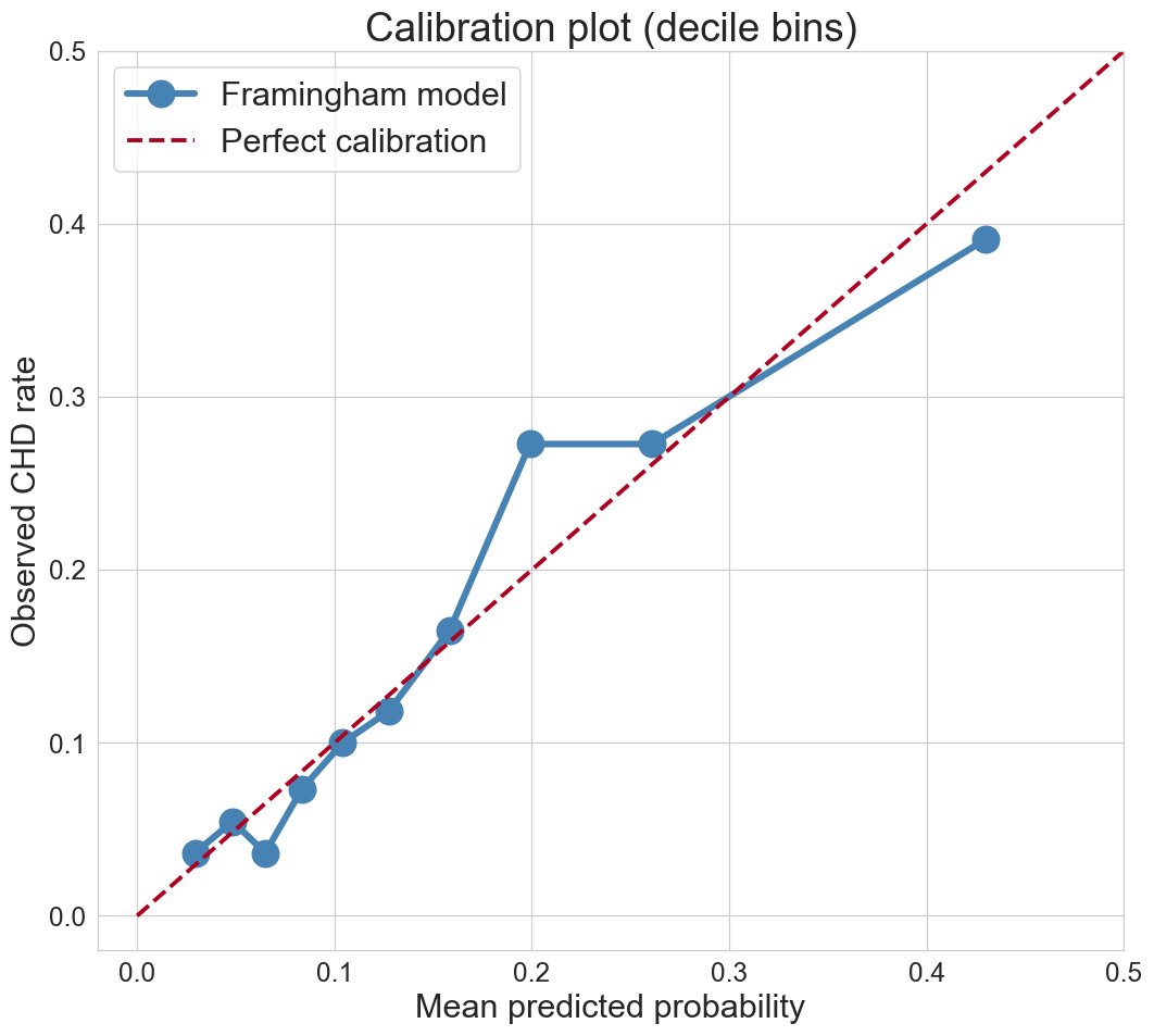
bin predictions into deciles

does “10% risk” mean 10% observed rate?

. . .

AUC measures ranking

calibration measures absolute probabilities

. . .

a model can have good AUC and bad calibration (or vice versa) — which matters depends on how you use the output

The last aggregate lie to unmask. Logistic regression outputs probabilities, not just classifications. But do those probabilities mean what they claim? If the model says “20% risk” for a group, do 20% of that group actually develop CHD? To check: bin predictions into deciles (10 equal-count buckets), compute the observed CHD rate in each bin, plot observed vs predicted. A perfectly calibrated model sits on the diagonal. Our model tracks the diagonal reasonably well across the range where most patients live. It’s well-calibrated — even though we just saw it fails badly on other dimensions. Calibration is orthogonal to ranking: AUC measures only the order of predictions (rescale and AUC is unchanged); calibration depends on the actual values. A model that outputs “0.20” for patients truly at 0.40 risk has perfect ranking but awful calibration. If you use probabilities directly for cost-benefit tradeoffs, calibration matters. If you just pick top-k patients to screen, only ranking matters.

back to the readmissions hook

the question that opened the lecture

a hospital’s model is “85% accurate” — deploy it?

now you know what to ask:

• what’s the baseline? (accuracy trap)
• what’s precision and recall at the chosen threshold?
• ROC curve — is the chosen threshold a good point on the tradeoff?
• does the model work across all patient groups?
• are the probabilities calibrated?

Close the loop. We opened with a hospital’s 85% accurate readmissions model. Now you have the toolkit to diagnose it. First, check the baseline — is “predict none” 85%? If so, accuracy alone tells you nothing. Next, look at precision and recall at whatever threshold is being used. Then the full ROC curve and AUC to see performance across thresholds. Then subgroup breakdowns — is the model equally good across age, race, insurance type? Finally, calibration — if the model says “40% readmission risk,” is it really 40%? The hospital’s decision on where to operate on the precision-recall curve is a cost-benefit call about intervention dollars, staff availability, and patient outcomes — not a statistics question.

key takeaways

• accuracy is misleading with imbalanced classes — check the baseline first
• the loss function determines what the model finds: logistic loss penalizes confident wrong answers
• gradient descent on a convex loss finds the global minimum (unique when the data isn’t separable)
• precision / recall reveal what accuracy hides — the right threshold is a cost-benefit call
• AUC summarizes ranking across thresholds; calibration checks absolute probabilities
• always check subgroup performance — aggregate metrics hide local failures

Six takeaways. The first three are about building a classifier: loss design, optimization, fitting. The last three are about evaluating one. The thread through all six: don’t trust a single number. Every aggregate can lie, and the way you dig into the lie depends on how your downstream decision uses the model.

next time

• Chapter 8: bootstrap — quantify uncertainty in any estimate (accuracy, AUC, odds ratio, …)
• Chapter 12: formal inference on logistic coefficients (confidence intervals, p-values)
• Chapter 13: decision trees — same classification problem, very different model

Today closed Act 1. Act 2 opens with the bootstrap — a resampling tool that lets us put confidence intervals on any statistic, including today’s classification metrics. Then Chapter 12 returns to logistic regression to do formal inference on coefficients. And in Act 3, trees and forests extend classification to nonlinear decision boundaries.

one-minute feedback

1. what was the most useful thing you learned today?
2. what was the most confusing?

give feedback

Closing ritual (1 min). Students fill out the form before leaving — silent, individual, not a discussion. The feedback is read and drives the next round of edits. Keep the slide up until the room clears.