Lecture 5: Multiple Regression and Feature Engineering

MSE 125 — Applied Statistics

Madeleine Udell

Monday, April 13, 2026

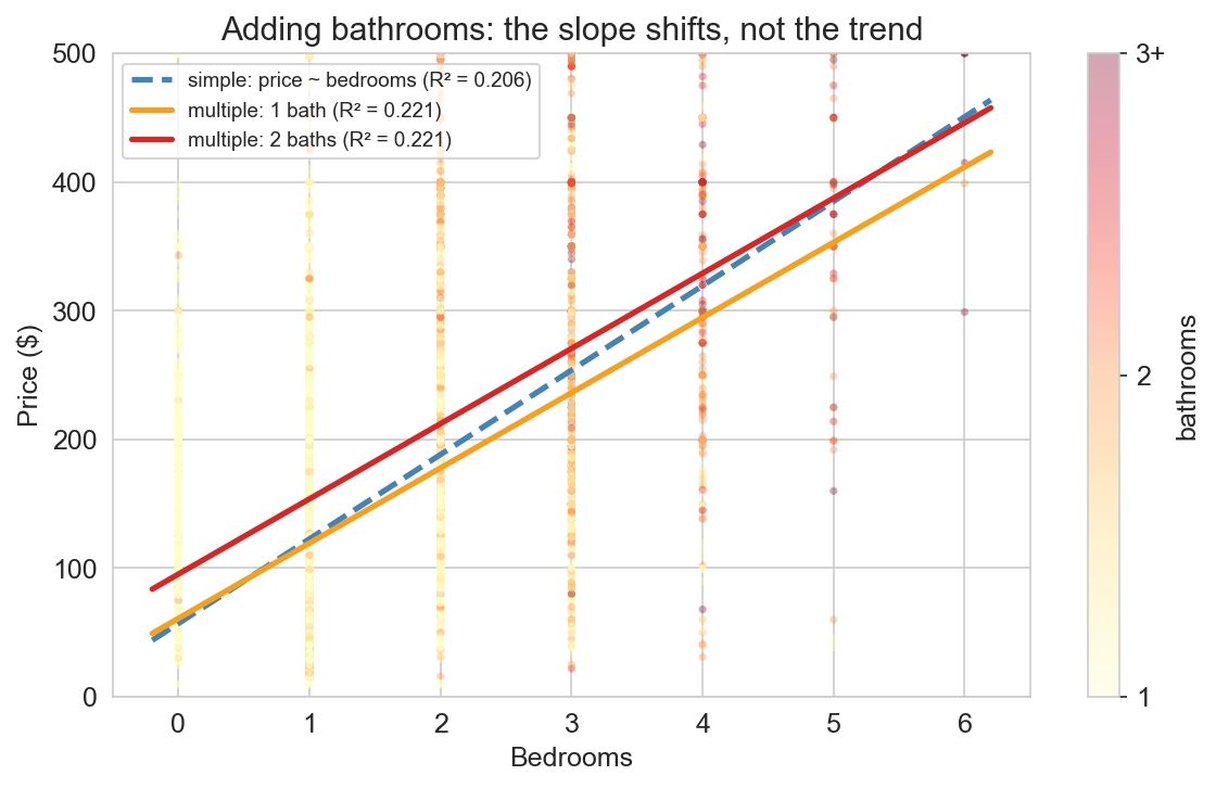
how much is a bathroom worth?

The hook. An Airbnb host is thinking about adding a second bathroom. How much more should they charge per night? Last lecture we built a regression from the mean up and stopped at one feature — bedrooms. That model literally cannot answer this question: it doesn’t even know bathrooms exist. Jump right in.

a host has a question

an Airbnb host is adding a second bathroom

how much more should they charge per night?

chapter 4’s model doesn’t know bathrooms exist

Frame the question in one sentence. The Chapter 4 model used bedrooms alone — every pricing signal correlated with bedrooms got absorbed into that single coefficient. We’ll fix that today.

today

• multiple regression
• one-hot encoding
• feature engineering
• diagnostics

Four blocks. Multiple regression extends Chapter 4’s machinery to more than one feature. One-hot encoding lets us feed categorical data into the same matrix. Feature engineering — interactions, indicators, logs — is where domain knowledge enters the model. Diagnostics is how you catch your own mistakes.

multiple regression with numeric features

adding bathrooms

chapter 4: \(\widehat{\text{price}} = 57 + 66 \times \text{bedrooms}\)

add bathrooms:

\[\widehat{\text{price}} = 27 + 58 \times \text{bedrooms} + 34 \times \text{bathrooms}\]

a 2BR / 1BA listing: \(27 + 58(2) + 34(1) = \$177\)

a 2BR / 2BA listing: \(27 + 58(2) + 34(2) = \$211\)

Start from the Chapter 4 baseline: price = 57 + 66 × bedrooms, R² = 0.206. Add bathrooms as a second column and we get: price = 27 + 58 × bedrooms + 34 × bathrooms, R² = 0.221. The bedrooms coefficient dropped from $66 to $58 and a new $34 bathrooms coefficient appeared. Walk through the concrete prediction: a 2BR/1BA listing gets 27 + 116 + 34 = $177; adding a second bathroom adds $34. The scatter on the right colors points by bathroom count. The dashed blue line is simple regression; the solid lines are the multiple regression at 1 and 2 bathrooms. The vertical gap between lines is the $34/bathroom coefficient. (Note: the adding-bathrooms image still shows the old fit lines — acceptable for now, we’ll refresh if time permits.)

the feature matrix

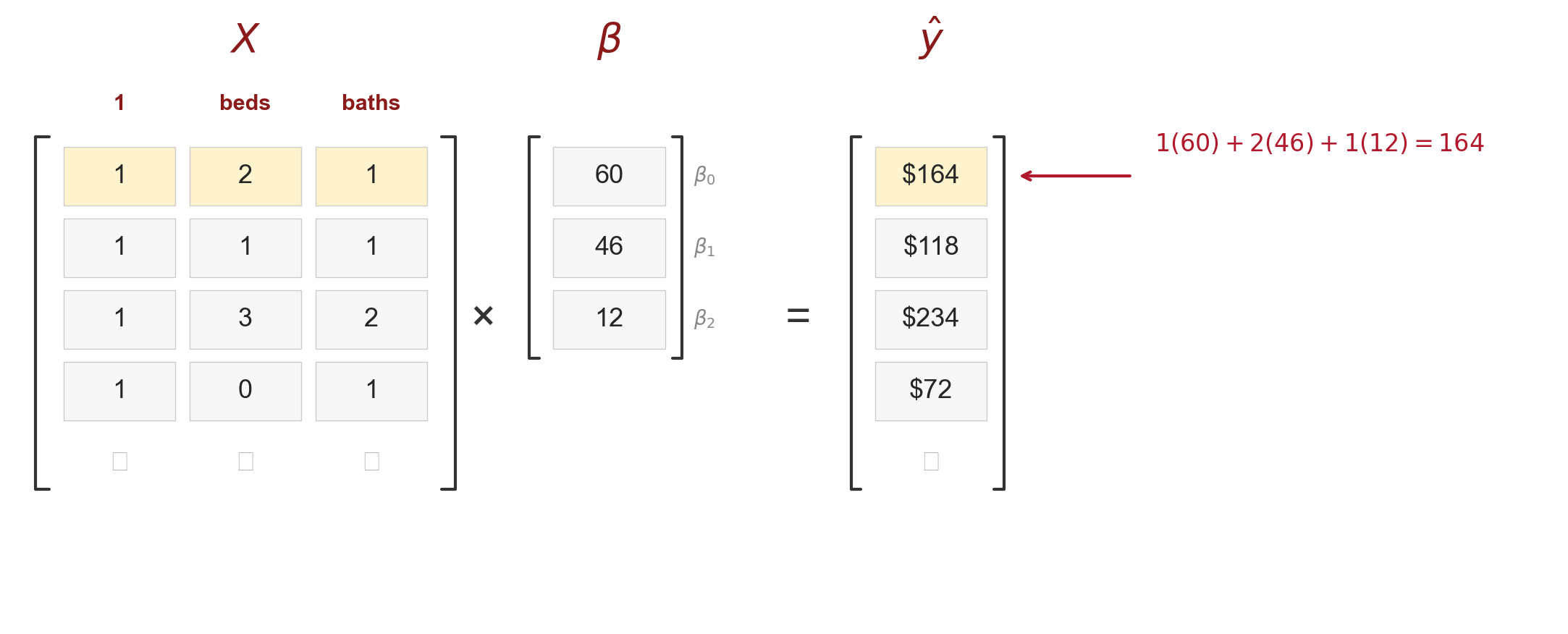
• each row of \(X\) = one listing
• each column = one feature (plus a column of ones)
• \(\widehat{y} = X\beta\) computes all predictions at once

The feature matrix is the bookkeeping object that lets us talk about all the features at once. The diagram shows how a single row of X times beta gives one listing’s prediction — students can trace through the multiplication and verify it gives the same equation we wrote on the previous slide. For the rest of the lecture, “adding a feature” means “adding a column to X.”

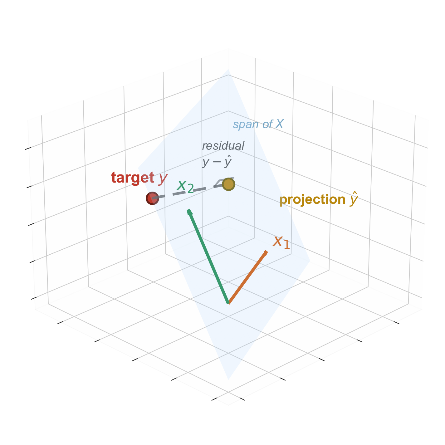
the span grows with more features

\[\text{span}(X) = \{X\beta : \beta \in \mathbb{R}^p\}\]

the set of all possible predictions · the span of the columns of \(X\)

• 1 feature + intercept: 2D plane in \(\mathbb{R}^n\)
• 2 features + intercept: 3D subspace
• more columns → bigger span → closer projection

Generalizing last lecture’s picture. With one feature and an intercept, the span was a 2D plane and the regression line was the projection of y onto that plane. The diagram on the right shows the 3D case: the light blue plane is the span of X, V1 and V2 are two feature directions, the red point is y (true prices), and the gold point is y-hat (the projection). The residual is the dashed perpendicular line from y down to y-hat. Each new feature adds one dimension to the span, so y-hat can only get closer to y.

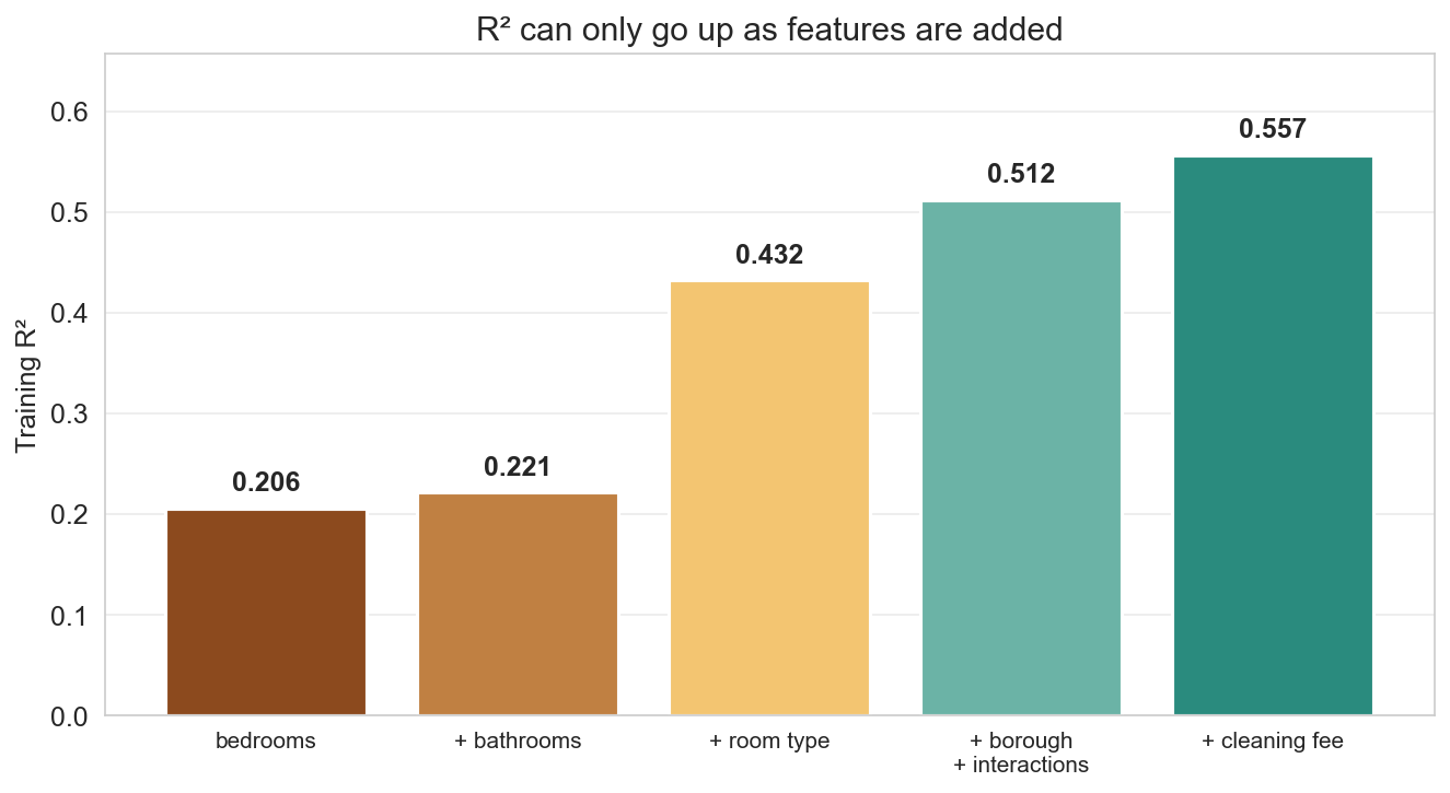
training R² can only go up

adding a feature never decreases training \(R^2\)

• new column → span grows (or stays)
• closer projection → higher \(R^2\)
• \(R^2_{\text{train}}\) is monotonic in # features

danger: \(R^2\) rewards you for adding noise

This is a fact about linear algebra, not about the data. With the current filter, R² climbs from 0.206 (bedrooms alone) → 0.221 (+ bathrooms) → 0.432 (+ room type) → 0.512 (+ borough + interactions) → 0.498 (+ cleaning fee + missing indicator) — each bar can only be taller than the last within a nested-feature sequence. The big jumps come from room type and borough, not from adding another numeric feature. It’s also the reason we can’t trust training R² as a model quality metric — Chapter 6 will formalize this with train/test splits. Note: the r2-staircase.png image still shows the old filter’s numbers (0.156 → 0.559); the shape is right, the individual values are stale.

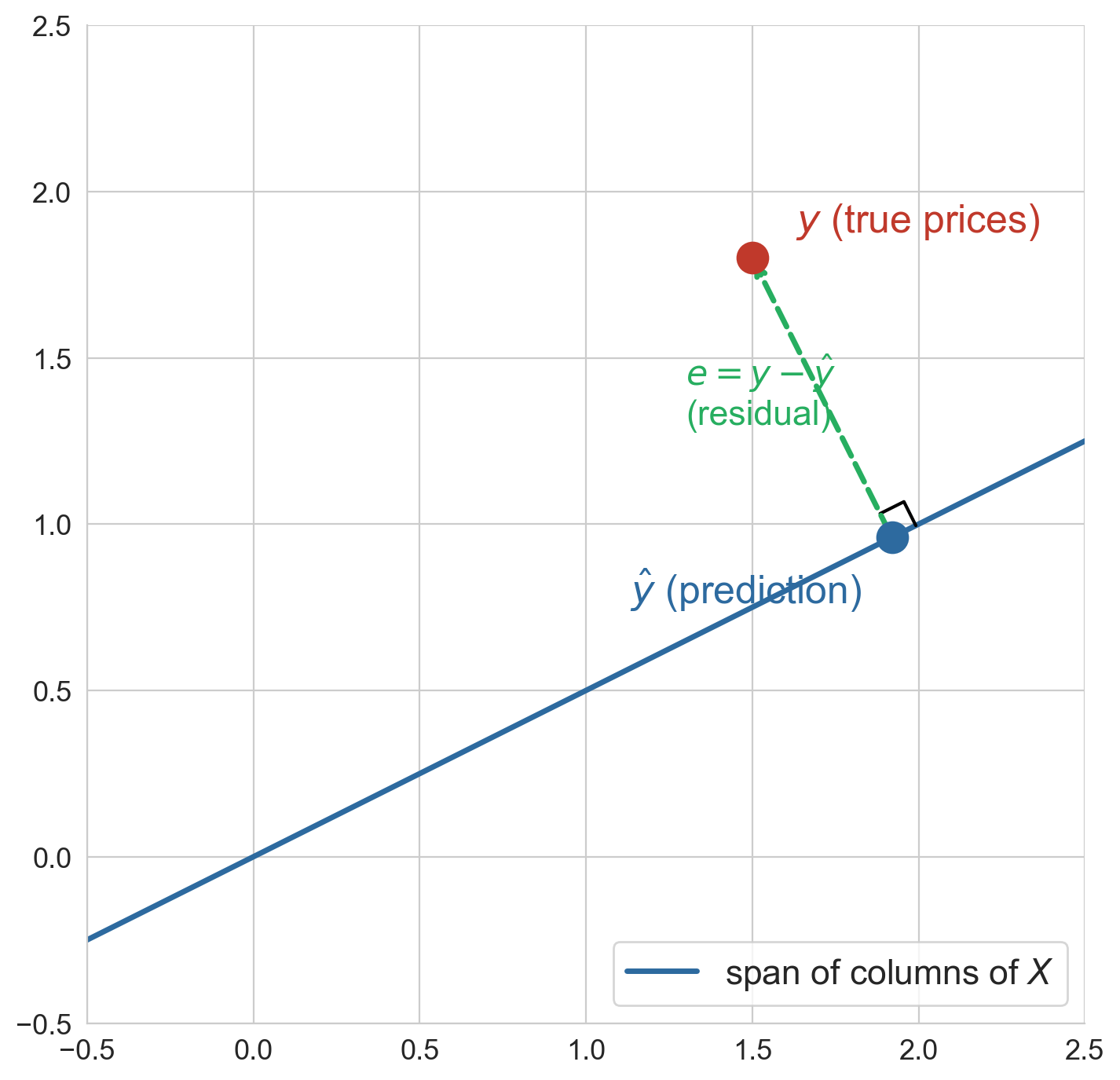
the normal equations

residual orthogonal to every feature column:

\[X^T \epsilon = 0 \quad \text{where } \epsilon = y - X\beta\]

rearrange:

\[X^T X \beta = X^T y\]

\[\widehat{\beta} = (X^T X)^{-1} X^T y\]

closed-form solution for the least-squares coefficients

Stack last lecture’s orthogonality conditions: residuals sum to zero (orthogonal to the ones column), no linear pattern with bedrooms (orthogonal to bedrooms column), no linear pattern with bathrooms (orthogonal to bathrooms column). All three live in one equation: X^T epsilon = 0. The diagram on the right is the same projection picture from Chapter 4: y (true prices) projects onto the span of X to give y-hat, and the residual e = y - y-hat is perpendicular to the span. The normal equations are the algebraic statement of that perpendicularity.

normal equations: code

X = np.column_stack([np.ones(n), bedrooms, bathrooms])
beta = np.linalg.solve(X.T @ X, X.T @ y)
print(beta)

[26.66 58.42 34.38]

• np.linalg.solve(A, b) — don’t invert; factor and solve
• matches LinearRegression().fit(...) exactly

Practical note: never compute (X^T X)^-1 explicitly. Use np.linalg.solve which factors the matrix and solves in one step — more numerically stable and faster. This matters when X^T X is ill-conditioned (multicollinearity, coming in part 5).

what does the coefficient mean?

\[\widehat{\text{price}} = 27 + \mathbf{58} \times \text{bedrooms}\] \[+ \; 34 \times \text{bathrooms}\]

coefficient = association holding bathrooms constant

The phrase “holding bathrooms constant” is the phrase of the day. The plot on the left shows only 1-bathroom listings — the slope through that filtered subset is about $58/bedroom, matching the multiple regression coefficient. The cards on the right show the model’s predictions for two specific listings that differ by one bedroom but share the same bathroom count. The $58 gap IS the coefficient. Informally: compare only listings with matching bathroom counts, then ask how much price changes with bedrooms. Say the phrase at least once out loud.

simple vs multiple

model	bedrooms coef
bedrooms only	$66
+ bathrooms	$58

bathrooms coefficient: $34

the bedrooms coefficient dropped $8 — why?

Just present the fact: adding bathrooms caused the bedrooms coefficient to drop from $66 to $58, and a new $34 bathrooms coefficient appeared. Don’t explain why yet — that’s the discussion question on the next slide.

why did the bedrooms coefficient drop from $66 to $58 when we added bathrooms?

if stuck: think about what a 3-bedroom apartment usually has

DISCUSSION: Think-pair-share (4 min) Prompt: “Why did the bedrooms coefficient drop when we added bathrooms?” Format: 30 sec think + 90 sec pair + 90 sec share If stuck: “A 3-bedroom apartment probably has how many bathrooms? A studio?” Key insight (draw out — this is the student’s phrase to arrive at, not yours): bedrooms and bathrooms travel together. Bigger apartments have more of both. In simple regression, the bedrooms coefficient absorbed part of what is really a bathrooms signal. Multiple regression disentangles the two by holding bathrooms constant. The word for this situation is confounding — reveal the word on the next slide after students have said “travel together” or “come as a package” out loud. Preview of Chapter 18 on causal inference. These are associations, not causal effects.

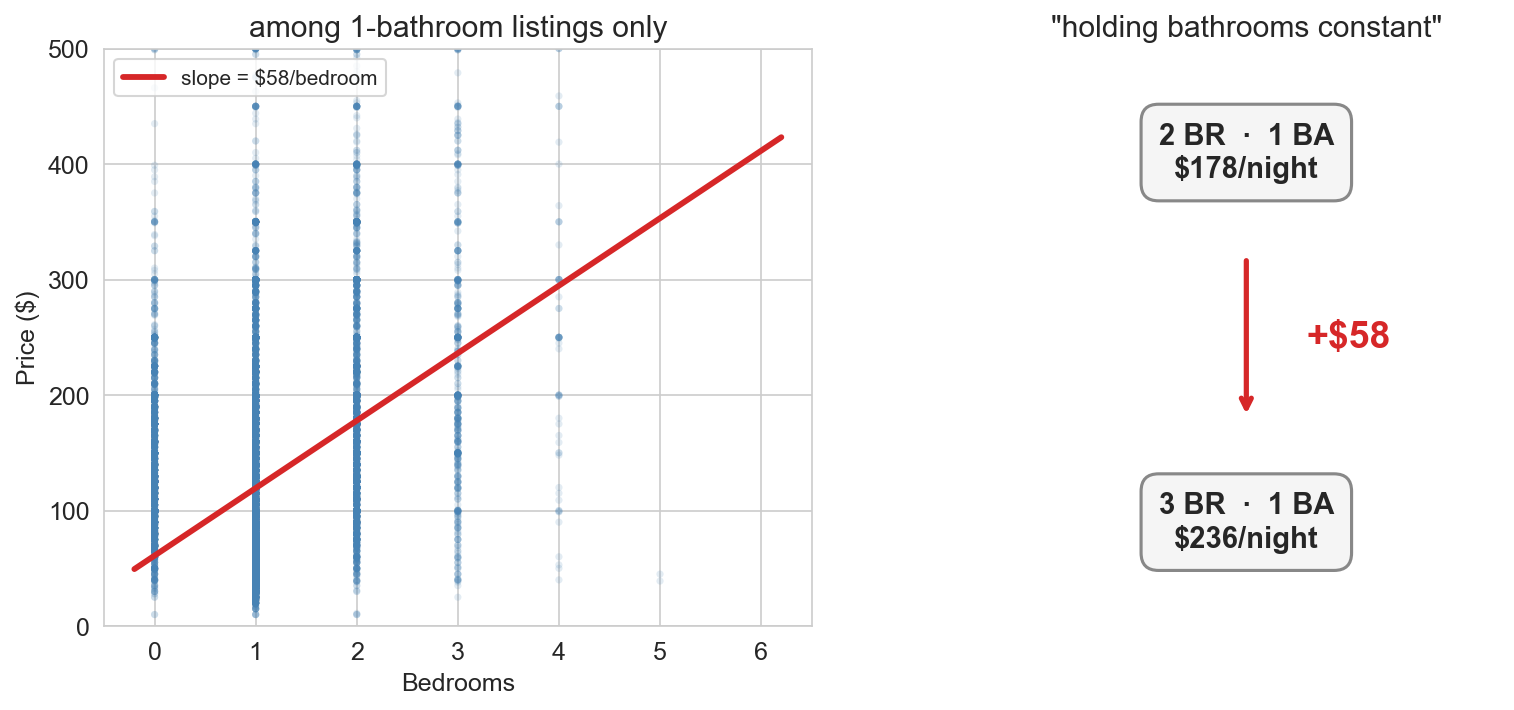
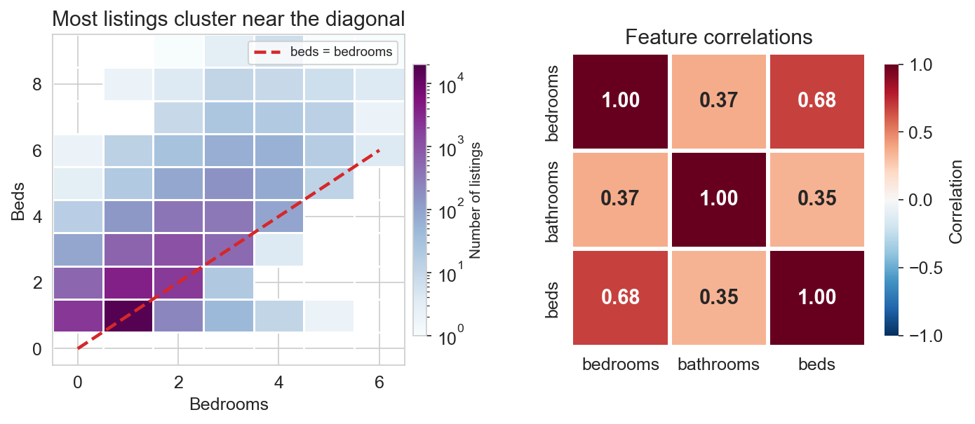
bedrooms and bathrooms travel together

simple regression on bedrooms alone absorbed part of the bathrooms signal

multiple regression disentangles them by holding each constant

these coefficients measure association, not causation

the word for this: confounding (→ Ch 18)

The slide title lands on the students’ own phrase from the discussion. Reveal the explanation one fragment at a time: (1) simple regression absorbed a signal that “really” belongs to bathrooms; (2) multiple regression disentangles by holding each constant; (3) these are associations, not causal effects — the biggest vocabulary point of Chapter 5; (4) the technical name is confounding, which returns in Chapter 18. The heatmap shows the correlation structure: bedrooms-bathrooms ≈ 0.37, bedrooms-beds ≈ 0.68. Avoid saying “the $8 drop is the confound” — that overclaims. Say “the $8 drop is what the multiple regression reassigns to bathrooms when it holds bedrooms constant.”

how do you put a string into a matrix?

the problem

df['room_type'].unique()
# ['Entire home/apt', 'Private room', 'Shared room']

you cannot multiply “Entire home/apt” by \(\beta\)

regression needs numbers

Room type is one of the strongest predictors of price — entire apartments cost more than private rooms. But it’s a string. We need a way to convert it to numbers without imposing a fake ordering.

how would you convert room type to numbers for regression?

if stuck: what about entire home = 2, private room = 1, shared room = 0?

DISCUSSION: Think-pair-share (3 min) Prompt: “How would you convert room type to numbers?” If stuck: “What does a linear model do with your numbers? It multiplies them by a coefficient and adds them up — what does that assume about the spacing between categories?” Advance the “if stuck” fragment only after the think-pair phase — it is a wrong-answer anchor, not a solution. Integer encoding is the most tempting wrong answer; surfacing it gives stuck students something concrete to react to. Key insight (draw out from the share phase): integer encoding forces an ordering AND equal spacing — the model treats “entire” as literally 2× “private.” We did not tell the data that. A correct answer is one binary column per category. That is one-hot encoding, on the next slide. Call on two or three students before moving on — the wrong answer has to land out loud before the right answer means anything.

one-hot encoding

one binary (0/1) column per category

pd.get_dummies(df['room_type'])

entire home	private room	shared room
1	0	0
0	1	0
1	0	0
0	0	1

each row has exactly one 1 — the category it belongs to

The mechanical step. The dummy columns are also called “indicator” variables. Every row gets exactly one 1 across the dummy columns — that’s what “one-hot” means. No fake ordering.

the dummy variable trap

three dummy columns sum to the all-ones vector

but the intercept column is the all-ones vector

• let \(e\) = entire, \(p\) = private, \(s\) = shared
• the columns are linearly dependent: \(e + p + s = \mathbf{1}\)
• \(X^TX\) is singular — no unique solution

A set of vectors is linearly dependent if one of them can be written as a combination of the others. Here the room-type dummies (entire e, private p, shared s) sum to the all-ones vector in every row — exactly the intercept column. So 1 - e - p - s = 0, and the four columns are linearly dependent. X^T X becomes singular and the normal equations have no unique solution. The fix is simple: drop one dummy.

reference level

Reference level

drop one category; its baseline is absorbed into the intercept. every other coefficient measures a difference from the reference.

pd.get_dummies(df['room_type'], drop_first=True)
# drops "Entire home/apt" (alphabetical first)

Q: if we dropped “Shared room” instead, which coefficients would change?

A: all of them — the baseline shifts

The dropped category is the baseline. All other coefficients are interpreted relative to it. Which category you drop doesn’t change predictions (y-hat is identical), but it does change how you read the coefficients — every remaining coefficient is a difference from whichever category you dropped. Ask the question out loud before advancing the fragment. If students are stuck, remind them that the intercept absorbs the baseline, so changing the baseline means the intercept changes too. The predictions are identical; only the story told by the coefficient table changes.

room type alone

Intercept (Entire home/apt baseline):  $186
  room_type_Private room:              −$108
  room_type_Shared room:               −$129

• intercept ≈ mean price of entire homes
• private room: $108 less than an entire home
• shared room: $129 less than an entire home

The intercept here is the baseline price for an entire home. Private and shared rooms are priced relative to that baseline — both negative, as expected. Values from rendered book: intercept = $186, private room ≈ -$108, shared room ≈ -$129 (from the stand-alone room_type-only model).

the full model

price ~ bedrooms + bathrooms + room type

Intercept:                  $80.79
bedrooms:                  +$43.67
bathrooms:                 +$43.13
room_type_Private room:    −$95.77
room_type_Shared room:    −$119.77
R² = 0.432

Present the coefficients first without the payoff — let students read the table. The intercept dropped from $186 (room-type-only) to $81 once bedrooms and bathrooms entered, because part of what the room-type intercept was absorbing was really “entire homes tend to have more bedrooms and bathrooms.” R² = 0.432. Numbers verified from the rendered book. The next slide is the cinematic callback to the opening hook.

how much is a bathroom worth?

about $43 more per night

holding bedrooms and room type constant

Callback to the opening hook. The opening asked “how much is a bathroom worth?” — now we can answer it: about $43/night, holding bedrooms and room type constant. Not $100, not $200. Say “association, not effect” explicitly — pre-Chapter 18 discipline.

coefficients, visualized

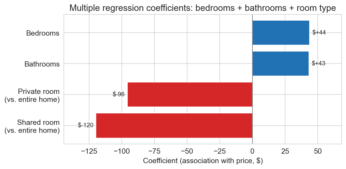
negative bars = discounts from the entire-home baseline · intercept = $81 (the entire-home baseline)

Q: compute the predicted price of a private room, 2 bedrooms, 1 bathroom

\(81 + 44(2) + 43(1) - 96 = \$116\)

The coefficient bar chart from the book. The two biggest magnitudes are the room-type discounts, not the continuous features. Domain knowledge is paying off. After the chart lands, run a verbal computation check: ask the class to compute the private-room / 2BR / 1BA prediction out loud before advancing the final fragment. This demotes the former 2-min discussion slide into an inline 45-second mechanical check — it tests whether students can read a coefficient table without burning a full discussion slot. Common mistakes to watch for: forgetting the intercept, or subtracting $96 the wrong way.

linear in parameters, not in features

the big idea

every model we’ve fit: \(\widehat{y} = X\beta\)

• linear in \(\beta\) — yes, always
• linear in \(x\) — not required

the columns of \(X\) can be anything we compute from the raw data

This is the key reframe of feature engineering. People hear “linear model” and think it can only fit straight lines. Wrong. It fits straight lines in the span of whatever X you hand it. You can put in x², log(x), x₁·x₂, or a sentiment score derived from listing text. The math doesn’t care.

interaction terms

is an extra bedroom associated with the same price change in Manhattan and the Bronx?

\[\widehat{y} = \beta_0 + \beta_1 \text{beds} + \beta_2 \mathbf{1}_{\text{Manh}} + \beta_3 (\text{beds} \times \mathbf{1}_{\text{Manh}})\]

where \(\mathbf{1}_{\text{Manh}} = 1\) if Manhattan, \(0\) otherwise

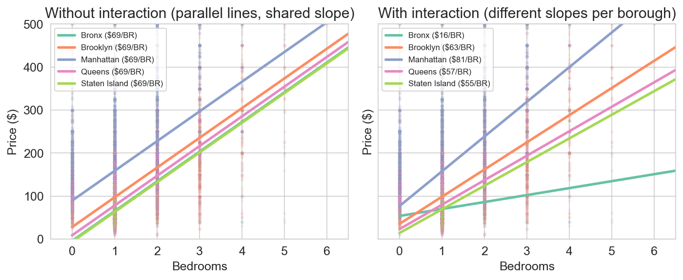
left: without \(\beta_3\) — parallel lines · right: with \(\beta_3\) — slopes differ by borough

Interactions let one feature’s association with the response depend on another. The product of two columns is just another column you compute and add to X — still linear in beta. Left panel: pooled model price ~ bedrooms + borough_dummies forces every borough to share the same $69/BR slope; only the intercept varies. Right panel: interaction model with bedrooms × borough terms — each borough sets its own slope. The Bronx is the outlier at $16. The actual per-borough numbers are on the next slide.

borough-specific bedroom slopes

borough	$/bedroom
Manhattan	$81
Brooklyn	$63
Queens	$57
Staten Island	$55
Bronx	$16

a bedroom in Manhattan is associated with ~5× more than a bedroom in the Bronx

Per-borough slopes from the interaction model. Manhattan leads at $81/bedroom. Brooklyn, Queens, and Staten Island cluster in the $55-$63 range. The Bronx is the outlier at $16 — a bedroom there is associated with a much smaller price increase. A model without interaction terms hides this heterogeneity inside a single pooled $69/BR coefficient. Numbers verified from the rendered book.

missing values as features

df['cleaning_fee_imputed']  = df['cleaning_fee'].fillna(0)
df['fee_missing']           = df['cleaning_fee'].isna().astype(int)

• ~19.6% of listings leave the cleaning fee blank
• missing fee = host bundles cost, skipped field, or expects guest to tidy up
• impute with zero — missing contribution reads directly as \(\hat{\beta}_{\text{missing}}\)
• indicator column fee_missing flags imputed rows

About one in five listings has no cleaning fee. A blank fee might mean the host bundles cleaning into the nightly rate, skipped optional fields, or expects guests to tidy up — we don’t know from the data alone, but the pattern predicts price. Median price when missing: $85 vs $110 when present. Impute with zero: a missing row contributes beta_fee × 0 + beta_missing × 1 = beta_missing to the prediction — a single clean number. Any other imputation constant gives identical predictions (the indicator absorbs the offset), but zero makes the coefficient easiest to read.

the missing indicator earns its place

Q: does the indicator column add anything beyond the imputed fee?

baseline (no fee):             R² = 0.4322
+ imputed cleaning fee:        R² = 0.4845
+ imputed fee + fee_missing:   R² = 0.4982

cleaning_fee_imputed:  $0.80 per $1 of fee
fee_missing:          +$35.71

a blank fee carries its own price signal — missingness is information

Inline predict-then-reveal. Ask the class the question verbally before advancing the fragment — wait for 1-2 guesses. Then reveal the three-way R² comparison. The imputed fee pushes R² from 0.432 to 0.484 — a big jump. The fee_missing indicator adds a smaller bump (0.484 → 0.498). Small, but real. Read the coefficients: a missing-fee row contributes beta_missing ≈ $35.71; a median-fee ($50) row contributes beta_fee × 50 ≈ $40.04. The model has learned that the pattern of missingness carries a price signal that raw imputation alone can’t capture. The arithmetic comparison (~$4 cheaper) lives in the book — stay on the big idea here.

a hint hiding in the interaction coefficients

dollars vary · percentages cluster

borough	$/bedroom	% per bedroom
Manhattan	$81	51%
Brooklyn	$63	64%
Queens	$57	71%
Staten Island	$55	80%
Bronx	$16	23%

four of five boroughs cluster 51–80% per bedroom · Bronx is the outlier

if one shared percentage replaces five dollar slopes, one coefficient does the work of five

Convert the interaction-model dollar slopes into percentage jumps per bedroom. Dollars span a 5× range — $16 in the Bronx to $81 in Manhattan — so the interaction model needs a separate slope for each borough. Percentages tell a different story: Manhattan 51%, Brooklyn 64%, Queens 71%, Staten Island 80% — much closer to “one shared number” than the dollar column. Only the Bronx (23%, $16) fits neither picture, and it will be the outlier we accept as the price of simplification. If we can find a model that speaks in percentages, one coefficient can do what five interaction terms were doing. The log transform is that model. This slide is clue #1.

a second clue: the fat right tail

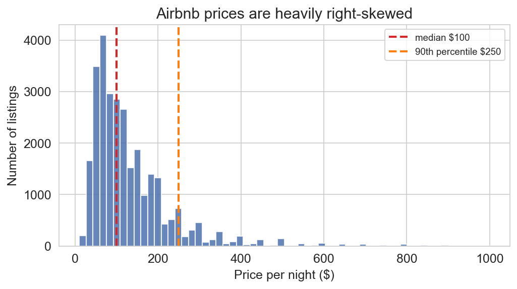
median $100 · 90th percentile $250 · tail runs to $999

the top 5% of listings hold nearly half the level model’s squared error

a $50 miss on $100 (50% off) ≡ a $50 miss on $500 (10% off) — squared dollars can’t tell them apart

Clue #2 is in the price distribution itself. The histogram is heavily right-skewed — median $100, 90th percentile $250, tail all the way to $999. When a level model fits by minimizing squared dollar error, the tail dominates the error budget: the top 5% of listings account for nearly 50% of total squared error, almost 10× their fair share. The reason: squared-dollar error treats a $50 miss on a $100 listing (a disaster) the same as a $50 miss on a $500 listing (mild). We want an error metric that treats proportional mistakes on equal footing. That is what a log transform does — and it is the same move the interaction-coefficient hint suggested. Both clues point to the same fix.

a bedroom is worth more in a luxury apartment

linear model: each bedroom adds a fixed dollar amount

• adding a bedroom to a luxury loft is worth more dollars
• adding a bedroom to a rundown studio is worth fewer dollars
• few large Airbnbs exist — they command a disproportionate premium

prices grow multiplicatively, not additively

Both clues point the same direction. The interaction coefficients said the model should think in percentages (clue #1). The fat right tail said the least-squares objective should too (clue #2). The fixed-dollar assumption breaks: adding a bedroom to a luxury Manhattan loft is worth more in absolute dollars than adding one to a small Bronx walk-up. The handful of large Airbnbs that can host a family reunion command a disproportionate premium because they fit large groups. The dollar response to “one more bedroom” grows with the base size — the super-linear pattern a straight line cannot match. Log transform captures both clues at once.

log transform straightens the curve

ax.set_yscale('log') — log y-axis, same data. level fit curves; log-level fit is straight.

Both panels show the same scatter with a log-scaled y-axis (semilogy). Left: the level fit price ~ bedrooms is a straight line in dollars but visibly bends on the log axis — it underfits the high-bedroom listings. Right: the log-level fit log(price) ~ bedrooms is a straight line on the log axis, matching the multiplicative pattern. The log model captures the super-linear bedroom premium that the level model has to fake.

multiplicative interpretation

model.fit(df[['bedrooms']], np.log(prices))
# β₁ = 0.33

\[e^{0.33} \approx 1.38\]

each bedroom multiplies price by ~1.38 — about 38% more per bedroom

On the log scale, a unit change in x corresponds to multiplying y by e^beta. For beta ≈ 0.33, that’s a factor of about 1.38 — each extra bedroom raises price by about 38%, proportionally. This matches intuition better than “each bedroom adds a fixed dollar amount no matter what.” Verified from the rendered book.

same multiplier, different dollars

log model with borough: shared multiplier per bedroom is about 1.42 (about 42%)

apply that multiplier to each borough’s base:

borough	$/bedroom (0→1)
Manhattan	$39
Brooklyn	$25
Queens	$21
Staten Island	$19
Bronx	$18

same proportional jump · bigger base → bigger dollars

honest limit: the Bronx is an outlier we accept — the price of simplification

The log-with-borough fit gives every borough the same multiplier (~1.42, about 42% per bedroom) but applies it to different base prices. Manhattan’s bigger base means a bigger dollar jump per bedroom. The log model expresses this borough heterogeneity with one extra coefficient per borough (just intercepts) instead of a fleet of bedrooms × borough interactions. Soft-tone framing of the Bronx: clue #1 already told us four of five boroughs cluster at 51–80% and the Bronx sits at 23% — the log model compresses five interaction slopes into one shared multiplier and pays for that compression by under-fitting the Bronx. We accept the outlier as the price of simplification, not as a modeling failure.

log on x: when \(x\) spans orders of magnitude

\[y \sim \log(x) \quad\Longrightarrow\quad \text{a **1% increase** in } x \text{ adds about } \tfrac{\beta_1}{100} \text{ to } y\]

use it when \(x\) ranges over orders of magnitude:

• square footage (200 vs 2,000)
• income ($30k vs $300k)
• city population (10k vs 10M)

a unit change in income means something totally different at the bottom and top — a percentage change is the natural unit

The third row of the four-combinations table. Use log on x when the raw feature spans orders of magnitude, so a percentage change is the natural unit of variation. For square footage, going from 200 to 201 sqft is nothing; going from 200 to 220 sqft (a 10% jump) is meaningful. The coefficient tells you how much y changes per 1% change in x — divide by 100 for the “per 1%” reading. Our Airbnb data has a couple of features like this: accommodates ranges from 1 to 16, and number_of_reviews spans zero to thousands. Neither is critical today — the main use of log on x is outside the Airbnb story, and the next slide uses accommodates for the clearest in-data example.

elasticity: \(\log(y) \sim \log(x)\)

Elasticity

when both \(y\) and \(x\) are on the log scale, \(\beta_1\) is the percentage change in \(y\) from a 1% change in \(x\).

\[\log(\text{price}) \sim \log(\text{accommodates}) \quad\Longrightarrow\quad \beta_1 \approx 0.66\]

a 10% larger listing is associated with about 6.6% more price

elasticities are dimensionless — compare effects across features on wildly different scales

The fourth row of the table, and the most important one for business students. Elasticity is what economists reach for when they want to compare the price sensitivity of demand across products, or wage response to education across countries, or any two features measured in different units. The key property: the elasticity is a pure number (percent per percent), so you can compare “bedroom premium” to “capacity premium” even though one is measured in integer bedrooms and the other in people. Concrete number: log(price) ~ log(accommodates) gives β₁ ≈ 0.66, so a 10% larger listing is associated with about 6.6% more price. Note that accommodates does span an order of magnitude in our data (1 to 16), so log on x is actually the right call here. Say “price elasticity of capacity” out loud once.

the four combinations

model	\(\beta_1\) means	example
\(y \sim x\)	unit change in \(x\) → \(\beta_1\) change in \(y\)	each bed adds $66
\(\log y \sim x\)	unit change in \(x\) → multiply \(y\) by \(e^{\beta_1}\)	each bed × 1.38
\(y \sim \log x\)	1% change in \(x\) → \(\beta_1/100\) change in \(y\)	10% sqft → $5 more
\(\log y \sim \log x\)	1% change in \(x\) → \(\beta_1\)% change in \(y\)	elasticity (e.g. 0.66)

Reference table — the cheat sheet students should remember. Each row is the “what does β₁ mean?” answer for one of the four combinations of log-on-y and log-on-x. Row 1 is the standard linear model from Chapter 4. Row 2 is the log-level model we just fit for bedrooms (e^0.33 ≈ 1.38). Row 3 (y ~ log x) is the percentage-change-in-x case from the previous slide. Row 4 (log-log) is the elasticity case, with our accommodates example giving 0.66. Students should recognize all four patterns in output and know how to interpret the coefficient without peeking.

when should the response be on a log scale?

for which of these would you use log(y)?

• housing prices
• test scores (0–100)
• household incomes
• body temperatures
• company revenues

DISCUSSION: Poll (3 min — quick hand poll, vote on each item). Prompt: “Which responses would you log-transform?” Format: Quick hand poll per item. If stuck: “Which ones are strictly positive? Right-skewed? Bounded above?” Key insight: Log is appropriate when the response is positive, right-skewed, grows multiplicatively, and has no natural upper bound. Prices, incomes, revenues — yes. Test scores (bounded 0-100) — no. Body temperatures (narrow range, near a fixed mean) — no.

diagnostics: how you catch your own mistakes

adjusted R²

training \(R^2\) never decreases with more features — even random noise

penalize for the number of features:

\[R^2_{\text{adj}} = 1 - \frac{(1 - R^2)(n - 1)}{n - p - 1}\]

where \(n\) = sample size, \(p\) = number of features

• useless feature ⇒ \(p\) grows, \(R^2\) barely moves
• adjusted \(R^2\) drops

Adjusted R² is a quick sanity check. It penalizes gratuitous features. It’s not a replacement for train/test validation — that’s Chapter 6 — but it flags the worst excesses on the training set itself.

multicollinearity

beds and bedrooms are nearly the same feature · correlation ≈ 0.68

	without beds	with beds
bedrooms	+58.43	+28.48
bathrooms	+34.37	+25.52
beds	—	+30.98
\(R^2\)	0.2215	0.2755

bedrooms coefficient cut in half from $58 to $28 — beds absorbed the signal

Adding beds modestly improves R² (0.22 → 0.28) but cuts the bedrooms coefficient in half, from $58 to $28, and bathrooms drops from $34 to $26 while beds picks up around $31. The redundant feature redistributes explanatory power between the two highly correlated columns — the individual numbers have lost their stable meaning. Correlation between bedrooms and beds is about 0.68, well above the 0.37 between bedrooms and bathrooms. Numbers verified from the rendered book.

symptoms of multicollinearity

• coefficients become large and unstable
• small changes in data → big swings in coefficients
• opposite signs, blown-up magnitudes
• \((X^TX)^{-1}\) is ill-conditioned: amplifies noise

predictions may still be fine — individual coefficients become uninterpretable

The critical distinction: multicollinearity hurts interpretation, not necessarily prediction. If all you want is y-hat, a collinear model can still be OK. If you want to say “bedrooms are associated with X dollars,” collinear columns make that claim unreliable.

residual diagnostic vocabulary

residual = observed − predicted: \(\epsilon_i = y_i - \hat{y}_i\)

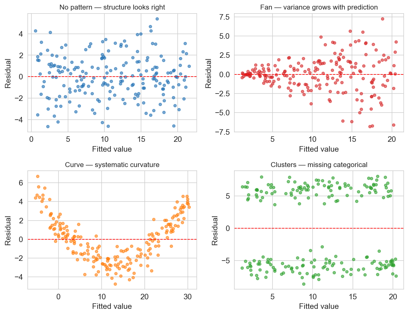
• fan → missing variance-stabilizing transform (often log)
• curve → missing polynomial or log feature
• clusters → missing categorical feature

The normal equations guarantee X^T epsilon = 0 — no linear pattern remains between features and residuals. Nonlinear patterns can still lurk, and when they do they are diagnosing something specific. Top-left is the reference: a well-specified linear model gives residuals that scatter evenly around zero. The other three panels are the misspecification vocabulary. Fan (top-right, variance grows with the prediction): the functional form is missing a variance-stabilizing transformation — often a log applied to y. Curve (bottom-left, U or arch shape): the true relationship has curvature the linear model cannot express; add a polynomial or log(x) feature. Clusters (bottom-right, vertically separated clouds): a categorical variable has been omitted. The next slide applies these three labels to our own Airbnb residuals.

Airbnb residuals: level vs log

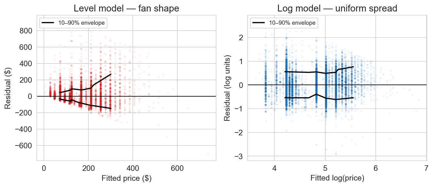
level model: fan from our vocabulary · spread grows with predicted price

log model: flat band · the fan is gone

The left panel is the fan from the synthetic vocabulary, staring back at us from real data. The 10–90% residual envelope widens from about ±$50 for cheap listings to ±$150 for expensive ones — the level model’s spread grows with its prediction, and the upper edge grows faster than the lower edge, matching the fat right tail from earlier. The right panel shows what happens when we transform y. The log-model envelope is nearly a horizontal band: residual spread is the same whether we’re predicting a $50 listing or a $500 one. Same data, same features — just a different target variable. The residuals told us which transformation we needed, if we had known what to look for.

what would you do next?

given the fan in the level-model residuals — fit the log model, or stay with level?

DISCUSSION: Think-pair-share (4 min — 60 sec pick a side, 90 sec share with a neighbor + what would you tell a host?, 60 sec debrief). Prompt: “Given the fan in the level-model residuals, fit the log model or stay with level?” If stuck: “Which model gives more honest uncertainty on a $500 prediction? Which gives more interpretable units to a host?” Key insight — draw out: Log model wins on residual structure and on the percentage interpretation that business stakeholders care about (a shared 42% premium per bedroom across all boroughs is one number, not five). Level model is still easier to explain to a non-technical audience and gives dollar coefficients directly. Either can be right — the residual plot is a diagnostic, not a verdict. The important thing is to look at the residuals before trusting the fit.

key takeaways

• multiple regression: more columns in \(X\), same projection math
• normal equations: \(X^TX\beta = X^Ty\)
• holding constant: coefficients are partial associations
• one-hot encoding: categories as binary columns with a reference level
• feature engineering: interactions, indicators, logs — all linear in \(\beta\)
• diagnostics: residual plots catch what \(R^2\) misses

The regression toolkit. Each bullet maps to one content block. Feature engineering is where domain knowledge enters the model — and it’s where most of the gains in practice come from.

what we still can’t answer

• is the $43 bathroom coefficient real or noise? → Chapter 12 (inference)
• does this model generalize to new data? → Chapter 6 (validation)
• does a bathroom cause higher prices? → Chapter 18 (causation)

we can fit models. next: how to trust them.

The three forward pointers. Chapter 6 is next — how do you tell if your model is overfitting? The answer will be train/test splits and cross-validation, which let us choose between models honestly instead of trusting training R².

logistics

• quiz 2 — this Wednesday (Apr 15) in class
• HW 2 — due Friday Apr 24
• read Chapter 6 (validation) before Wednesday

1 min. Quiz 2 is this Wednesday in class — same 2×2 format as quiz 1, covering regression through feature engineering. HW 2 (the Airbnb regression exercise) is already out and due Friday Apr 24 — remind students to start early. The reading for Wednesday is Chapter 6 on validation and the bias-variance tradeoff.

one-minute feedback

1. what was the most useful thing you learned today?
2. what was the most confusing?

give feedback

Closing ritual (1 min). Students fill out the form before leaving — silent, individual, not a discussion. The feedback is read and drives the next round of edits. Keep the slide up until the room clears.