Lecture 4: From the Mean to Simple Regression

Applied Statistics: From Data to Decisions

Professor Madeleine Udell

Wednesday, April 8, 2026

am I pricing this right?

A friend just put their first Brooklyn listing on Airbnb and texts: “am I pricing this right?” First instinct — charge the average. But the average knows nothing about the listing. Their place has two bedrooms; bigger places should cost more. Before you answer, you want a pricing model that reflects what you actually know about the listing. That’s what this chapter builds, in two stages: (1) ignore every feature and predict a single number (the mean), then (2) let the prediction respond to one feature (bedrooms) by fitting a line.

a friend’s Brooklyn listing

text from a friend: “just listed my 2-BR on Airbnb — am I pricing this right?”

first instinct: charge the average

but the average knows nothing about their listing

bigger places should cost more — can we do better?

This is the motivating scenario for the whole chapter. Stage 1: predict with no features (the mean). Stage 2: predict with one feature (bedrooms). Along the way: vectors, norms, projection, R².

today

• vectors in data: rows, columns, norms
• predicting with no features: the mean
• predicting with one feature: simple regression
• how good is the fit?: \(R^2\) and correlation
• regression to the mean

Quick agenda. Jump straight in.

vectors in data

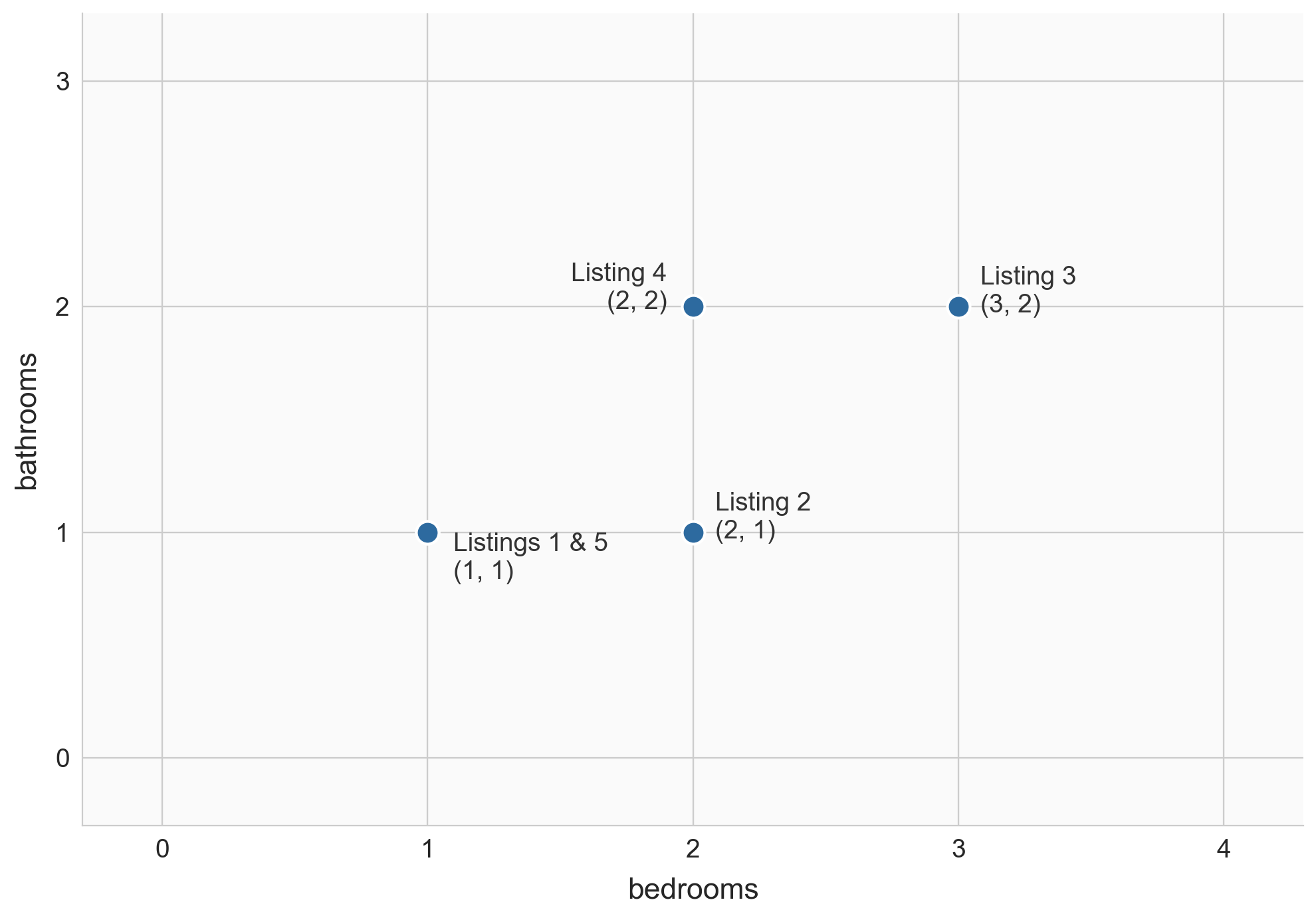
two views of a dataset

listing	bedrooms	bathrooms	price
1	1	1	100
2	2	1	150
3	3	2	250
4	2	2	200
5	1	1	120

• row view: each listing is a point in \(\mathbb{R}^d\) — listing 3 = \((3, 2, 250)\)
• column view: each feature is a vector in \(\mathbb{R}^n\) — bedrooms = \([1, 2, 3, 2, 1]\)

Two complementary views. Rows → points → similarity between listings. Columns → vectors → what a model can combine. Both matter today.

rows as points

nearby points = similar listings

Five listings plotted in bedroom/bathroom space. Listings 1 and 5 sit almost on top of each other. Listing 3 is farthest out.

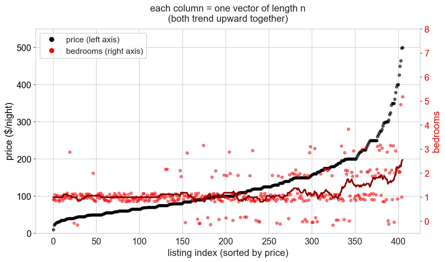
visualizing high-dimensional vectors

a column of \(n\) prices lives in \(\mathbb{R}^n\) — too many dimensions to draw as an arrow

index plot: plot value vs listing index

black = price, red = bedrooms (sorted by price) — they move together

The index plot is how we’ll visualize n-dimensional column vectors. Sort listings by price, then plot both columns on the same axes. When two vectors rise and fall together across listings, they “point” in the same direction in R^n. This visual agreement is what the inner product will measure.

difference vector

\[\text{listing 3} - \text{listing 1} = (3, 2) - (1, 1) = (2, 1)\]

tells us how they differ: +2 bedrooms, +1 bathroom

but how far apart as a single number?

The difference vector captures direction and magnitude of change. To collapse to a scalar, we need the norm.

norm = length of a vector

Norm

\(\|v\| = \sqrt{v_1^2 + v_2^2 + \cdots + v_n^2}\)

Pythagorean theorem in \(n\) dimensions.

np.linalg.norm([2, 1])
# sqrt(4 + 1) = 2.24

distance = norm of the difference: \(d(u, v) = \|u - v\|\)

The norm is just a generalized Pythagorean theorem. Distance between two vectors = norm of their difference.

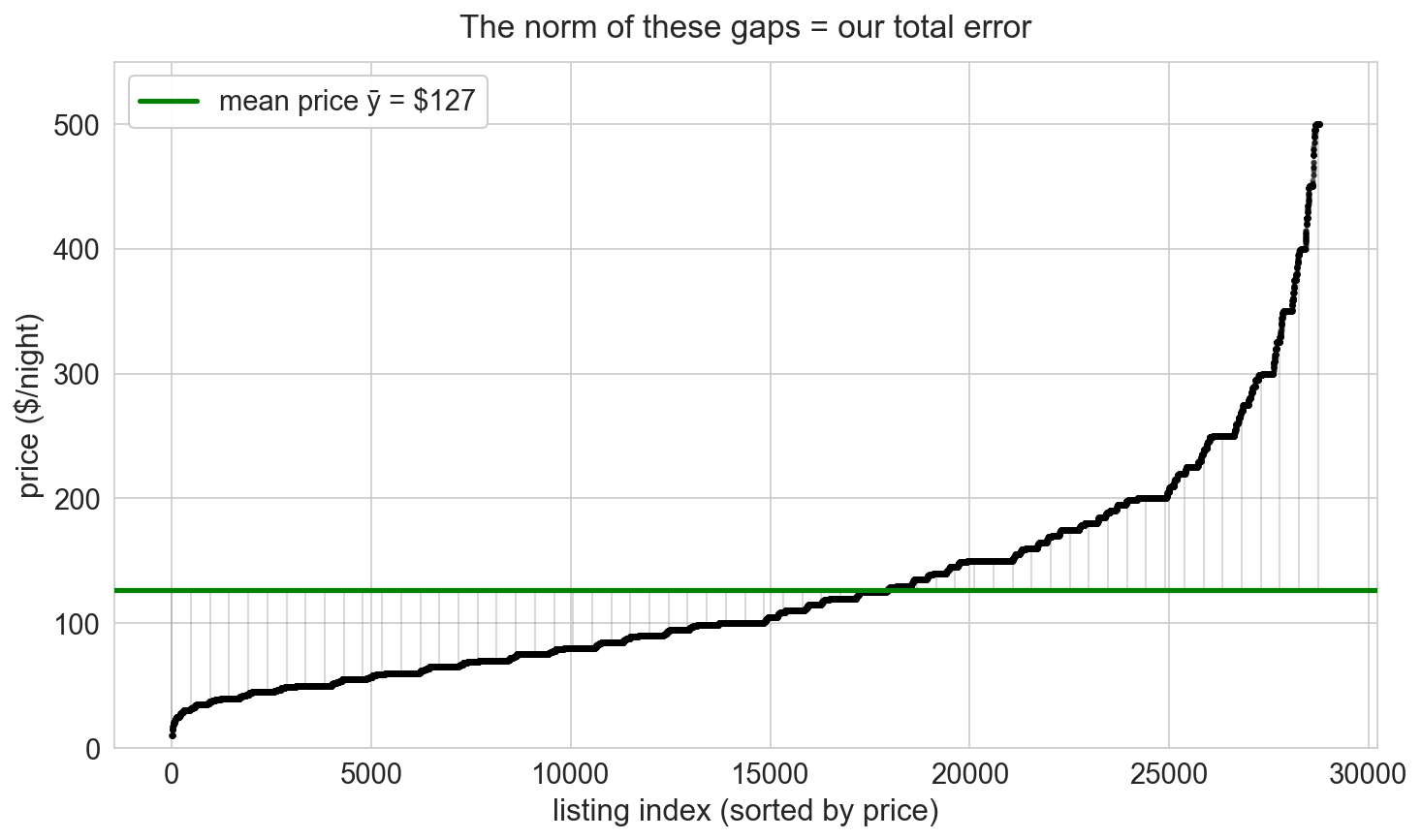
the norm will measure prediction error

predict every listing with a single number \(\widehat{y}\)

residual: \(\epsilon_i = y_i - \widehat{y}\) — one error per listing

\(\|\epsilon\|\) measures total prediction error

Preview of the geometry. Vertical segments from black dots (actual prices) to the green horizontal line (a constant prediction) are the residuals. Their norm is one number measuring how wrong we are overall. Our job is to make it small.

what does it mean for two Airbnb listings to be “similar”?

DISCUSSION: Think-pair-share (3 min — 30 sec think, 1 min pair, then share). Think: which features should count? Pair: do you agree on the same features? Share: what’s your definition of “close”? Prompt: “what does it mean for two listings to be similar?” If stuck: “if one is $100 and the other is $500, are they similar? what if the features match perfectly?” Key insight: “similar” depends on what you care about. Distance in feature space is one definition — but it weights every feature equally, and features with big numeric ranges dominate. This is why we’ll later normalize.

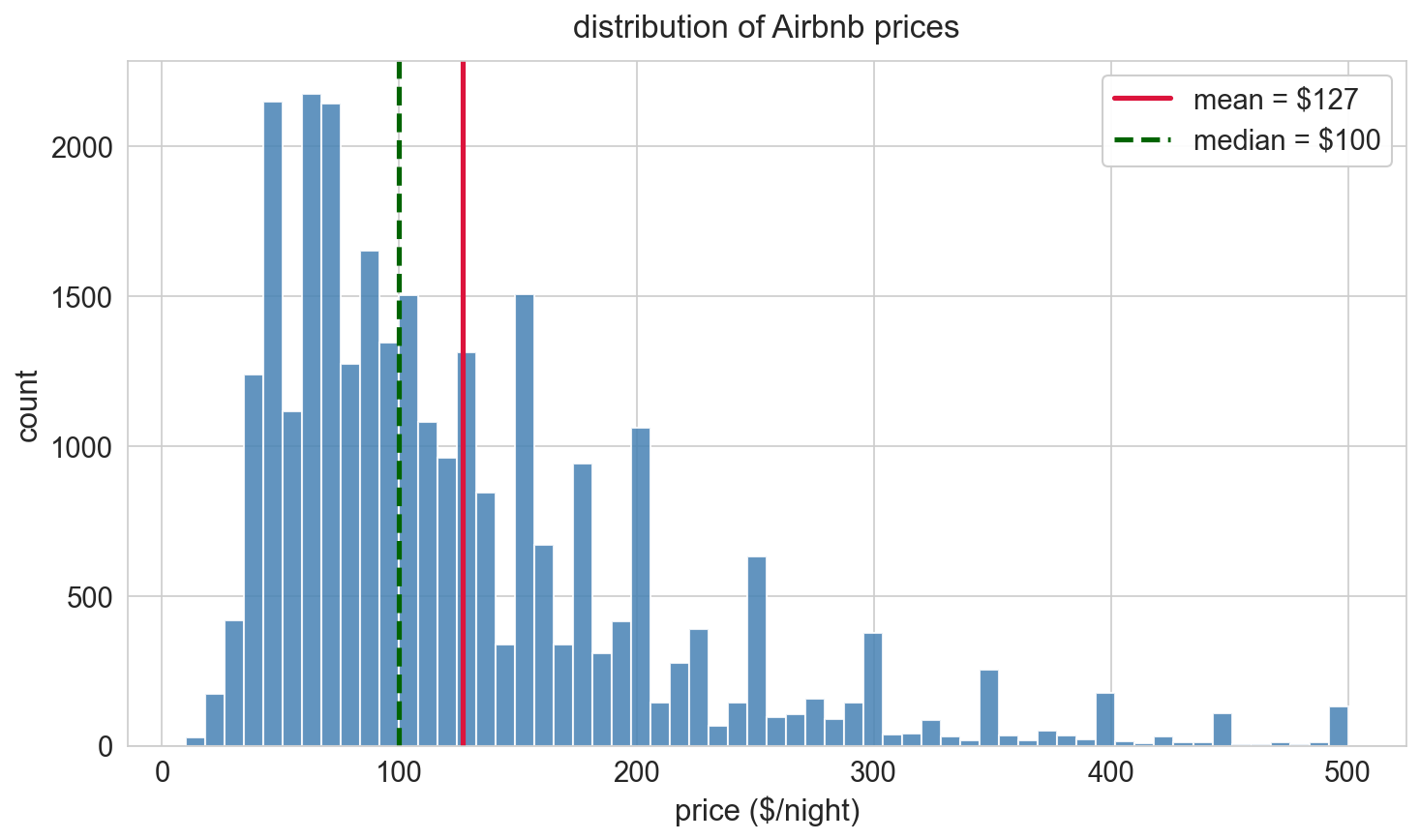
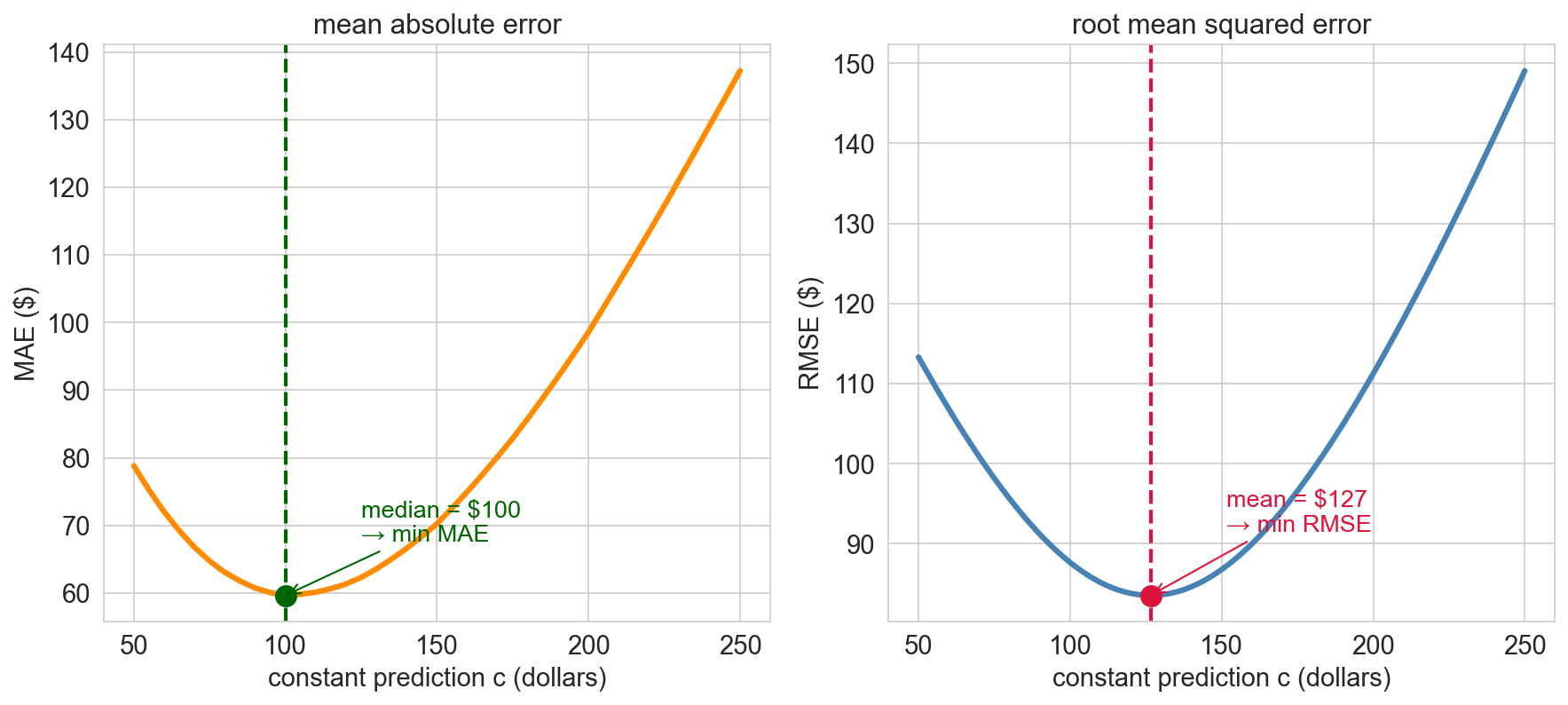
predicting with no features

the simplest predictor: a constant

\(n\) prices. what single number \(\widehat{y}\) should we guess for every listing?

Before any features, the simplest thing we can do: predict the same number for every listing. What should that number be?

two natural losses

minimize absolute error or squared error?

absolute → median; squared → mean

Left panel: sum of absolute deviations has V-shape, minimum at the median. Right panel: sum of squared errors is parabolic, minimum at the mean. Try the interactive widget in the book to explore this.

why should the mean win?

before the proof, a moment of reflection:

as \(c\) moves through the data, what happens to the derivative of \((y_i - c)^2\)?

why does that force a balance exactly at \(\bar{y}\)?

Reflection prompt before the calculus. Give students 20-30 seconds to think about why squared error pulls toward the mean. Each squared term contributes a linear derivative in c — summing them gives a linear function that crosses zero at the average. This is the intuition the proof formalizes.

why squared error gives the mean

\[\frac{d}{dc}\sum_i (y_i - c)^2 = -2\sum_i (y_i - c) = 0\]

\[\Longrightarrow \quad c = \frac{1}{n}\sum_i y_i = \bar{y}\]

the mean is the optimal constant predictor under squared error

Two-line calculus proof. Derivative is linear in c, so there’s a unique zero — at the mean. Later this same argument gives us the conditional mean: within any region of x, squared-error regression predicts the average of y in that region.

notation

Regression notation

• \(y = (y_1, \ldots, y_n)\) — response vector (actual prices)
• \(\widehat{y}\) — prediction vector
• \(\bar{y} = \frac{1}{n}\sum_i y_i\) — sample mean
• \(\epsilon = y - \widehat{y}\) — residual vector
• \(\beta_0\) — intercept

for the constant model: \(\widehat{y}_i = \beta_0\), and the best \(\widehat{\beta}_0 = \bar{y}\)

residuals sum to zero

when \(\widehat{y}_i = \bar{y}\):

\[\sum_i \epsilon_i = \sum_i (y_i - \bar{y}) = n\bar{y} - n\bar{y} = 0\]

in vector notation:

\[\mathbf{1}^T \epsilon = 0\]

the residual is orthogonal to the ones vector — our first normal equation

Remember this pattern — it generalizes. The best prediction makes the residual orthogonal to every feature used in the model. For the constant model, the only “feature” is the ones vector.

squared error → conditional mean

same argument, applied within each slice of \(x\):

squared-error regression estimates \(\mathbb{E}[Y \mid X = x]\)

(absolute error → conditional median; other losses → other summaries)

This is one of the most important properties of squared loss: the regression function estimates the conditional mean. The “best line” passes through the conditional means of y given x.

when should you predict with the mean vs the median?

• real estate prices: mean or median?
• insurance claims: mean or median?
• what’s the difference between “typical” and “average”?

DISCUSSION: Think-pair-share (3 min — turn to your neighbor for 2 min, then share). Prompt: “mean vs median — when does each win?” If stuck: “which is sensitive to outliers? which gives the right answer for a total cost estimate?” Key insight: Median is robust to outliers and answers “what’s a typical listing?” Mean answers “if I rent out every listing, what’s the average revenue per listing?” Squared error cares about total cost — you can’t ignore the $999 listings. This is why regression uses squared error, not absolute error.

predicting with one feature

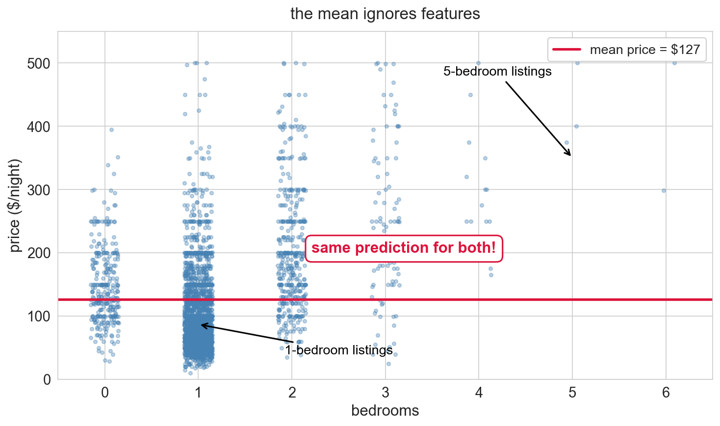
the mean ignores bedrooms

a 5-bedroom apartment and a studio get the same prediction

The mean gets the overall level right but misses the upward trend. Can we do better with bedrooms?

a linear combination of two columns

\[\widehat{y}_i = \beta_0 + \beta_1 \, x_i\]

\(\widehat{y}\) is a linear combination of \(\mathbf{1}\) and \(x\):

\[\widehat{y} = \beta_0 \, \mathbf{1} + \beta_1 \, x\]

The prediction is a weighted sum of two column vectors: the ones vector (scaled by the intercept) and the bedrooms vector (scaled by the slope). Different weights give different predictions.

the span: all reachable predictions

Span

\(\text{span}(\mathbf{1}, x) = \{\beta_0 \mathbf{1} + \beta_1 x : \beta_0, \beta_1 \in \mathbb{R}\}\)

all lines you could draw through the scatter plot

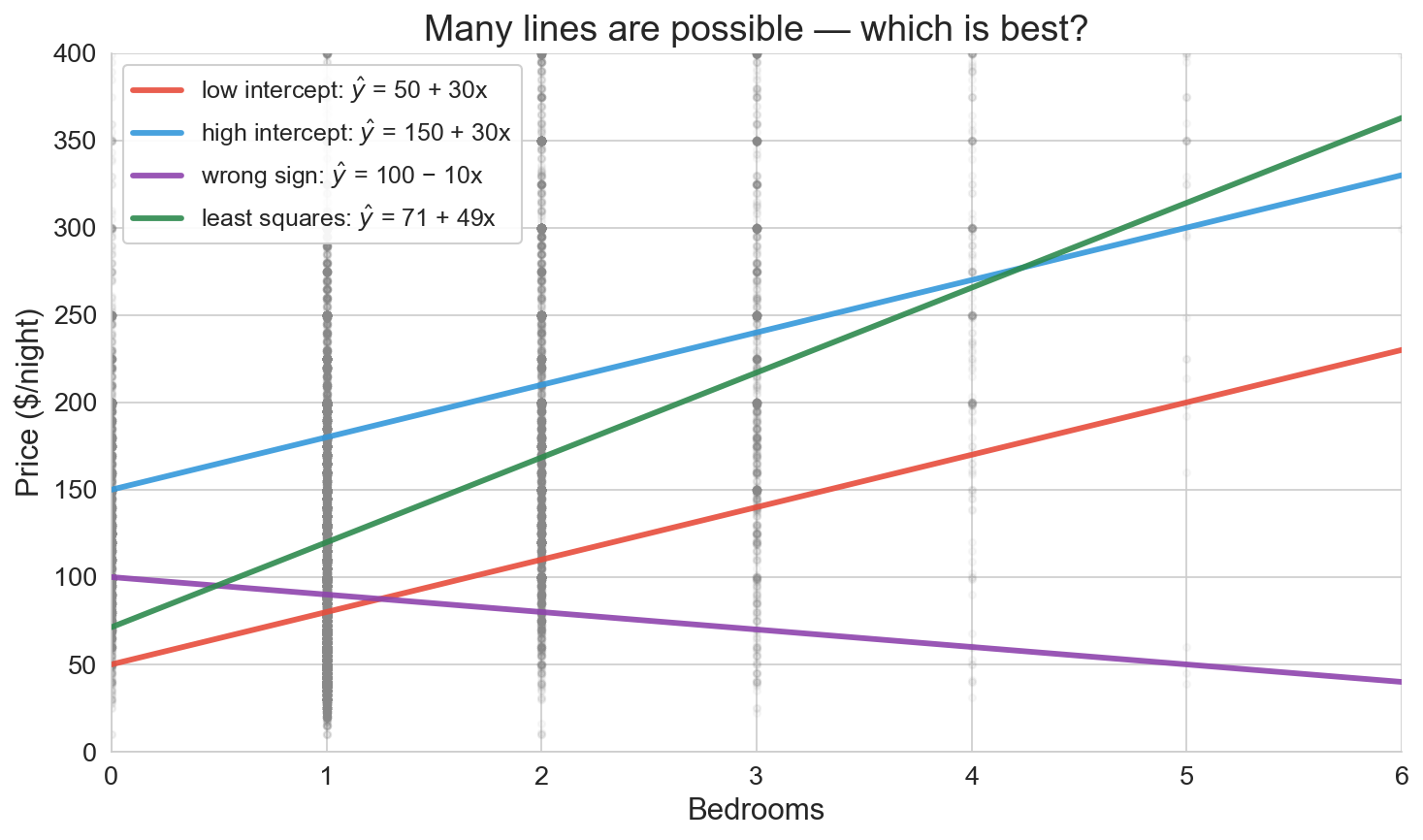
every \((\beta_0, \beta_1)\) traces a different line — which one is best?

Every choice of (β₀, β₁) traces a different line. The span of {1, x} is the set of all possible prediction vectors. Before we show candidate lines, we want students to commit to a criterion for “best.”

before you see any candidate lines: what would “best” look like?

DISCUSSION: Predict-then-reveal (2 min — 30 sec commit to a criterion, then reveal). Hint to deliver verbally: “passes through the middle of the cloud” is a starting point — make it precise enough that you could compute it. Prompt: “commit to a criterion for ‘best’ BEFORE seeing any lines.” If stuck: “close your left eye and imagine the vertical gaps from each point to a line.” Key insight: Most students land on ‘balances the gaps’ or ‘minimizes total error’ — that’s squared error, and it leads directly to projection. Now reveal the candidate lines.

many lines are possible — which is best?

• red, blue: too steep at the low end
• purple: slopes the wrong way
• green: closer but still arbitrary

we need a principled criterion — and it turns out to be geometric

Now the reveal. Walk through why each is wrong. The point: eyeballing isn’t enough. We need a principled definition of “best” — and the geometric view (projection) will give it to us.

switch to the column view

\(y\), \(\mathbf{1}\), and \(x\) all live in \(\mathbb{R}^n\) — one coordinate per listing

\(\text{span}\{\mathbf{1}, x\}\) = a flat plane floating in \(\mathbb{R}^n\)

every line you could draw = one point on that plane

the actual price vector \(y\) sits off the plane — no line fits every listing perfectly

Before showing the projection cartoon, get students to picture the column view. n listings → vectors in R^n. Span of two columns = a 2D plane inside that high-dimensional space. Every regression line is a point on the plane. The data vector y lives off the plane. Now the question becomes: which point on the plane is closest to y?

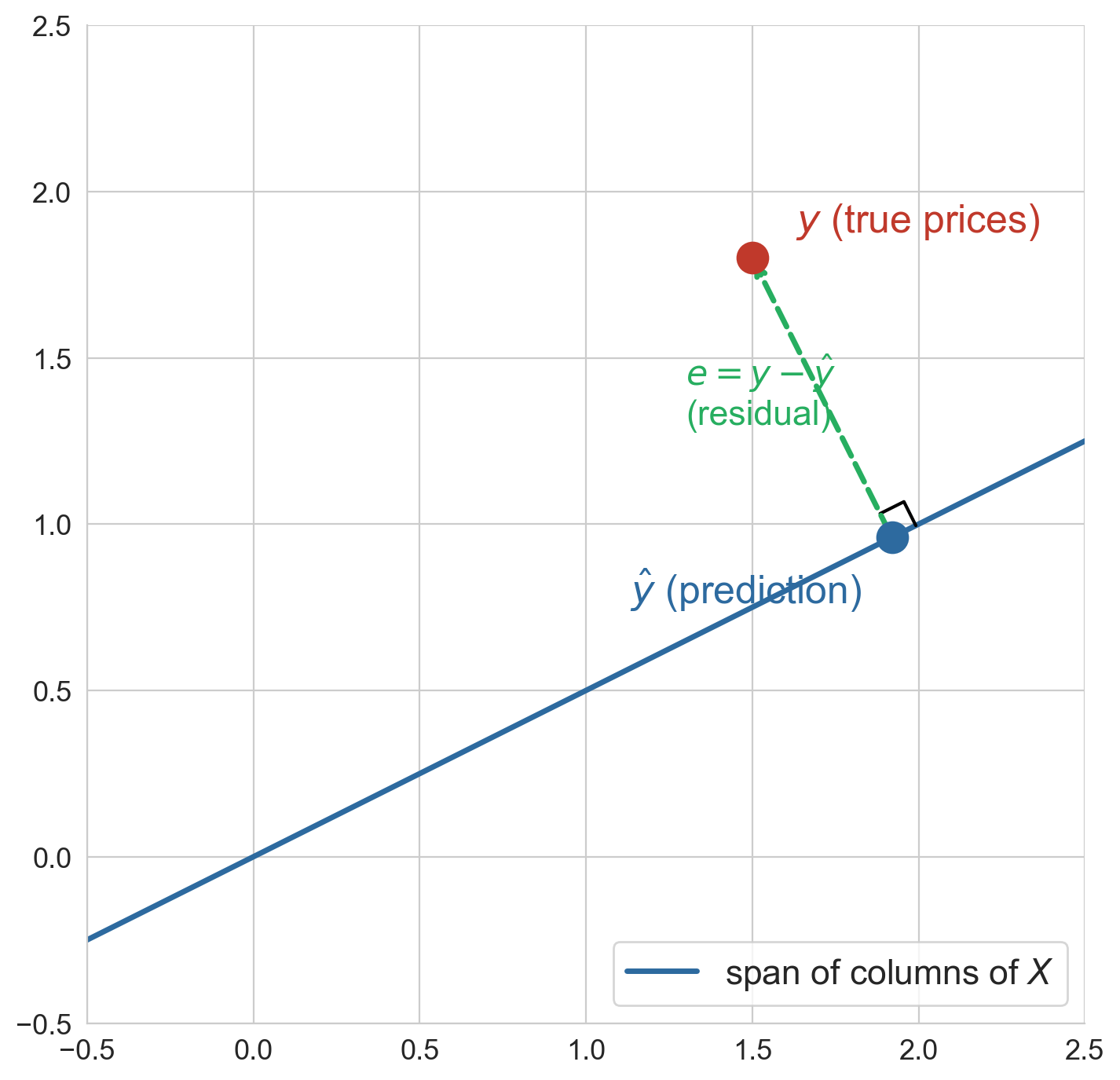
the geometric view: projection

• \(y\) is a point in \(\mathbb{R}^n\)
• \(\text{span}\{\mathbf{1}, x\}\) is a plane through the origin
• the closest point in the plane is the best prediction
• the residual \(\epsilon\) is perpendicular to the plane

Here’s the geometric heart. y is a point. The span of the features is a plane. The prediction ŷ lives in the plane — it’s a linear combination of the columns. The best ŷ is the point in the plane closest to y. Shortest distance from a point to a plane = perpendicular. That perpendicularity is the defining property of least squares.

the inner product

Inner product (dot product)

\(u^T v = \sum_{i=1}^n u_i v_i\)

• positive → same direction
• zero → orthogonal
• negative → opposite directions

take \(u = (1, 0)\) along the x-axis:

• \(u \cdot (1, 1) = 1\) → acute angle
• \(u \cdot (0, 1) = 0\) → right angle
• \(u \cdot (-1, 0) = -1\) → opposite

price and bedrooms both trend up → large positive \(y^T x\)

The inner product makes “perpendicular” precise. Zero inner product = orthogonal. The small 2D examples ground the rule: sign of the inner product tracks the angle. Callback to the index plot: if two columns rise and fall together, their inner product is positive and large.

orthogonality = best fit

the best prediction makes the residual orthogonal to every feature:

\[\mathbf{1}^T \epsilon = 0 \qquad \text{and} \qquad x^T \epsilon = 0\]

• first: residuals sum to zero (same as the mean model!)
• second: residuals have no remaining linear pattern with \(x\)

if some feature still aligned with the residual, you could reduce error by adjusting its coefficient

Two orthogonality conditions pin down the unique best line. The principle is the same as for the mean, just one more condition. If x^T ε were nonzero, we could absorb some of that pattern into the slope — so at the optimum, it must be zero.

normal equations

Normal equations (simple regression)

\(\mathbf{1}^T \epsilon = 0 \quad \text{and} \quad x^T \epsilon = 0\)

where \(\epsilon = y - \beta_0 \mathbf{1} - \beta_1 x\)

— the algebraic form of “residual orthogonal to features”

these two equations determine the unique \((\widehat{\beta}_0, \widehat{\beta}_1)\)

Two equations, two unknowns. The normal equations are just the orthogonality conditions, written out. Every regression problem reduces to solving a system like this.

the projection picture

\(\widehat{y}\) = orthogonal projection of \(y\) onto \(\text{span}\{\mathbf{1}, x\}\)

the right angle is why it’s the best fit

Clean version of the diagram. Perpendicular = shortest. This is the defining property of least squares.

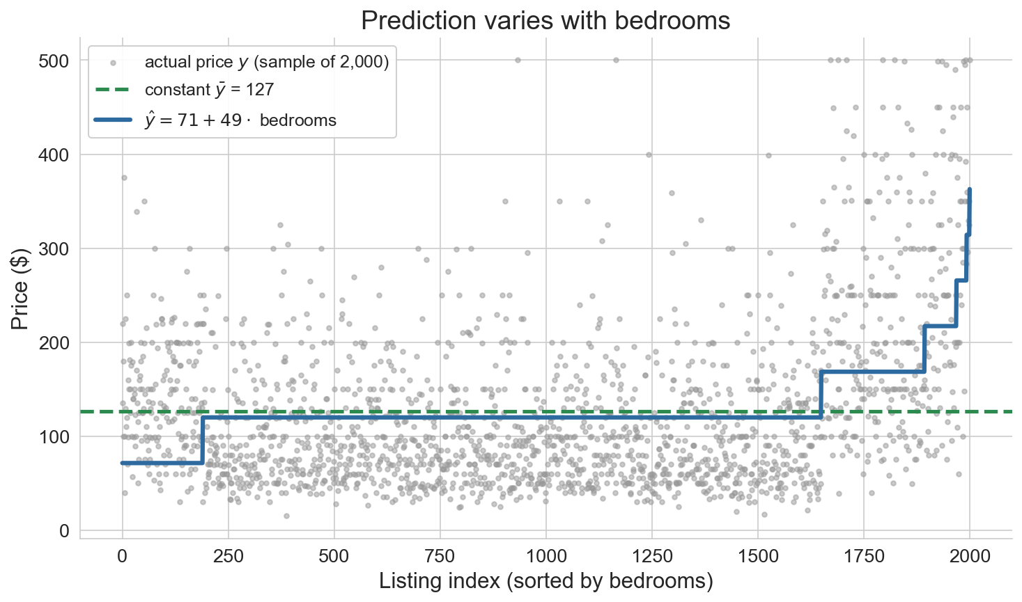
simple regression on Airbnb

model = LinearRegression()
model.fit(df[['bedrooms']], prices)

28,778 listings

ŷ = 71 + 49 × bedrooms
R² = 0.156

\[\widehat{y} = 71 + 49 \times \text{bedrooms}\]

The full NYC Airbnb dataset, filtered to prices in [$10, $500]. One feature, closed-form solution via the normal equations. R² = 0.156 — bedrooms alone explain about 16% of the variation.

interpreting the coefficients

\[\widehat{y} = 71 + 49 \times \text{bedrooms}\]

• intercept $71: predicted price for a studio (0 bedrooms)
• slope $49: each additional bedroom → $49 more per night

association, not causation — larger listings differ in many ways

The intercept is the base price of a studio. The slope says each additional bedroom is associated with $49 more per night. But bigger apartments differ in many ways from smaller ones — location, amenities, quality. We can’t say “adding a bedroom causes $49.” We’ll revisit this seriously in Chapter 18.

plug in a few listings

\[\widehat{y} = 71 + 49 \times \text{bedrooms}\]

listing	prediction
studio	$71
1-bedroom	$120
3-bedroom	$217
5-bedroom	$314

back to our friend’s 2-BR: model predicts $169/night

Concrete numbers make the model tangible. Plug bedrooms into the formula and read off predictions. For the 2-BR: 71 + 49 × 2 = 169. Our friend now has a starting anchor — though we’ll refine it with more features in Ch 5.

verify orthogonality

y_hat = model.predict(df[['bedrooms']])
residuals = prices - y_hat
np.dot(residuals, np.ones(len(df)))     # ≈ 0
np.dot(residuals, df['bedrooms'].values) # ≈ 0

residuals · 1       :  -0.0000  ✓
residuals · bedrooms:  -0.0000  ✓

the errors have no linear pattern left that bedrooms could capture

Both dot products are effectively zero — the normal equations are satisfied. This is guaranteed by the math. What is NOT guaranteed is that residuals look like random noise — we’ll check that with residual plots in Chapter 5.

what would a curved pattern in the residual plot mean?

DISCUSSION: Think-pair-share (3 min — 30 sec think, 1 min pair, then share). Think: if residuals vs bedrooms showed a U-shape… Pair: what’s the model missing? Share: how would you fix it? Prompt: “what does a curved residual plot tell us?” If stuck: “the orthogonality condition says residuals are uncorrelated with bedrooms linearly. What kind of pattern would still satisfy that?” Key insight: A U-shape would mean the true relationship is nonlinear — a quadratic term would help. Forward pointer to feature engineering (Ch 5): we can add bedrooms² as a new column and the same orthogonality machinery still works.

how good is the fit?

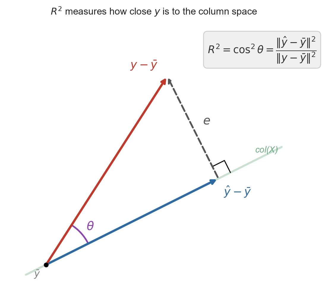
\(R^2\): fraction of variance explained

\(R^2\) (coefficient of determination)

\[R^2 = 1 - \frac{\|\epsilon\|^2}{\|y - \bar{y}\|^2}\]

• \(R^2 = 0\): no better than predicting \(\bar{y}\)
• \(R^2 = 1\): perfect fit

for our Airbnb regression: \(R^2 = 0.156\)

R² compares the model’s error to the baseline of always predicting the mean. Bedrooms alone explain about 16% of the price variation — the other 84% will need more features.

correlation

Correlation (Pearson’s \(r\))

\(r(u, v) = \dfrac{(u - \bar u)^T(v - \bar v)}{\|u - \bar u\|\,\|v - \bar v\|}\)

inner product of centered, length-normalized vectors.

• \(-1 \le r \le +1\)
• \(r = 0\) → centered vectors are orthogonal
• unitless: rescaling \(u\) or \(v\) doesn’t change \(r\)

Center each vector (subtract its mean), normalize to unit length, take the inner product. That’s correlation. It measures the angle between the centered vectors — pure direction, no units. Rescaling or shifting either input leaves r unchanged.

\(R^2 = r(y, \widehat{y})^2\)

Pythagorean theorem (centered \(y\)):

\[\|y - \bar{y}\|^2 = \|\widehat{y} - \bar{y}\|^2 + \|\epsilon\|^2\]

\[R^2 = \frac{\|\widehat{y} - \bar{y}\|^2}{\|y - \bar{y}\|^2} = r(y, \widehat y)^2\]

the first ratio is the correlation between \(y\) and \(\widehat{y}\), by definition

After centering, y, y-hat, and the residual form a right triangle with y as the hypotenuse. R² is the squared ratio of the leg (centered y-hat) to the hypotenuse (centered y) — and that ratio is exactly the correlation r(y, y-hat) between centered y and centered y-hat, by definition. R² measures how much of y lives in the feature span.

\(R^2 = r^2\) in simple regression

r = df['price'].corr(df['bedrooms'])
# r = 0.3944
model.score(df[['bedrooms']], prices)
# R² = 0.1556 = r²

for one predictor: \(R^2\) is literally \(r\) squared

(with multiple predictors, only \(R^2\) applies)

0.3944² ≈ 0.1556. R² = r² is only true for simple regression. With multiple predictors there’s no single r to square — we have to compute R² directly.

regression to the mean

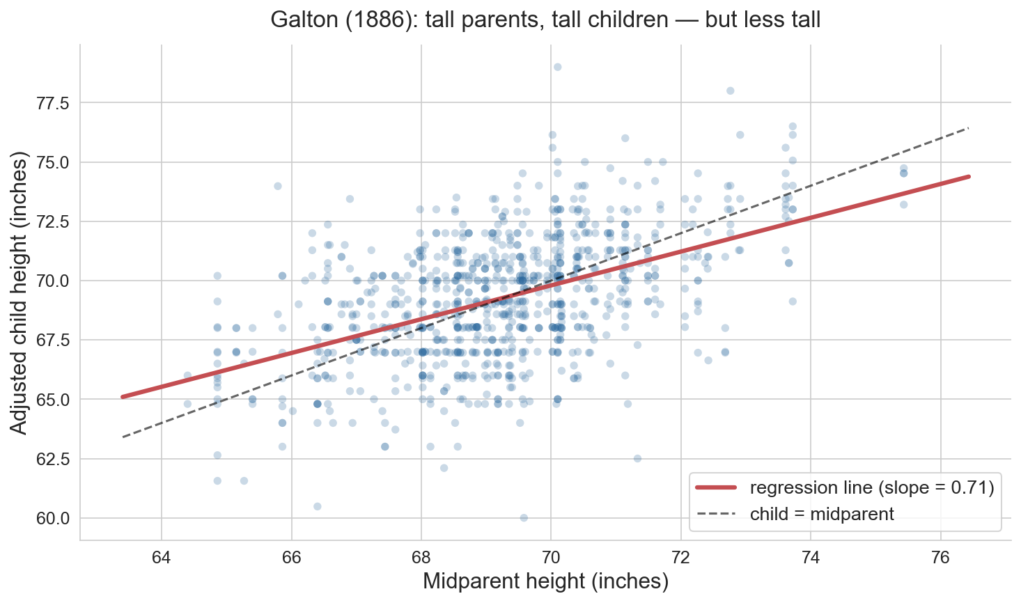
Galton’s heights

Francis Galton, 1886: tall parents → tall children, but less tall

934 children, 205 families: \(r \approx 0.50\), slope \(\approx 0.71\) (Galton’s own estimate: 2/3)

Galton’s actual 1886 dataset — 934 adult children from 205 families. He multiplied female heights by 1.08 to put everyone on a common male scale, then plotted each child against the “midparent height” (average of father and 1.08 × mother). The regression line is flatter than the 45-degree line (child = midparent). Parents 2 SD above average have children predicted to be only about r × 2 SD above average — pulled toward the mean. Galton himself estimated the slope at about 2/3, which is close to what we find. This is a purely statistical phenomenon, not biological. For the full story, see Salsburg, The Lady Tasting Tea, Ch. 4.

why “regression”?

since \(|r| < 1\), predicted \(y\) is always closer to \(\bar{y}\) (in SDs) than \(x\) is to \(\bar{x}\)

Galton called this “regression toward mediocrity” — the name stuck

purely statistical, not biological or causal

The phenomenon comes from imperfect correlation, not from any physical force pulling things toward the average. Extreme values are partly signal, partly luck — and luck doesn’t persist.

where else do you see regression to the mean?

• a team wins 90% of games one season. next year?
• a student scores in the 99th percentile. next exam?
• a player scores 45 points (season avg: 25). next game?

why does this keep happening?

DISCUSSION: Predict-then-reveal (3 min). Prompt: “regression to the mean in the wild” If stuck: “how much of an extreme outcome is skill vs luck?” Key insight: Any time performance is skill + noise, the best predictor after an extreme event is somewhere between the extreme and the long-run average. Coaches who bench a player after one bad game, or overpay after one great game, are ignoring this. The “Sports Illustrated jinx” is regression to the mean, not a curse.

skill + luck, luck resets

90% win rate = part skill, part luck

next season: the skill carries over, the luck resets

99th percentile exam = real knowledge + a run of favorable questions

knowledge holds; favorable run does not

whenever \(|r| < 1\), extremes on one measurement look less extreme on the next

The mechanism in every case is the same: observed performance = underlying ability + noise. The ability carries over; the noise doesn’t. Not “the team got worse” — just that an unusual streak has no reason to persist. Same logic for exam scores, stock picks, player performance, business quarters. This is not a curse, not a jinx — just algebra.

key takeaways

• two views of data: rows = points, columns = vectors in \(\mathbb{R}^n\)
• the mean is the best constant predictor under squared error
• simple regression is the orthogonal projection of \(y\) onto \(\text{span}\{\mathbf{1}, x\}\)
• residual ⊥ features: the defining property of least squares
• \(R^2 = r(y, \widehat{y})^2\): how much of \(y\) lives in the feature span
• regression to the mean: extremes don’t persist

The conceptual chain: vectors → mean → simple regression → projection → R². Each step adds one feature and one orthogonality condition.

what we can’t answer yet

\[\widehat{y} = 71 + 49 \times \text{bedrooms} \qquad R^2 = 0.16\]

• what about bathrooms? room type? neighborhood?
• can more features make \(R^2\) bigger?
• how do we encode categorical features?

next time: multiple regression (Chapter 5)

Forward pointer. Same orthogonality principle scales to any number of features. More columns → bigger span → closer projection. We’ll also transform raw data into features a linear model can use.

logistics

• read Chapter 4 before next lecture
• HW 1 due Friday April 10
• quiz 2 next Wednesday — covers Lec 4–5

one-minute feedback

1. what was the most useful thing you learned today?
2. what was the most confusing?

give feedback